Classical candlestick charting suffers from two mathematical flaws. First, it discretizes continuous four-dimensional (O, H, L, C) price excursions through discontinuous boolean thresholds. Second, it triggers patterns unconditionally without reference to institutional liquidity zones. This paper establishes the econometric foundations of the Daily Trading Opportunity (DTO) model inside 4CastMachine AI. Using continuous-time extreme-value variance estimators (Parkinson, Garman-Klass, Rogers-Satchell, and Yang-Zhang), we prove that full OHLC tuples carry 7.4x to 14x higher asymptotic statistical efficiency than close-only series. We also show why two-bar fused candles (D2) improve directional signal-to-noise ratio by +41.4%. Next, we formulate volatility-normalized bar coordinates scaled by ATR across five smooth DTO dimensions: Trend Bias (Market Strength), Momentum Excursion (RoCT), Structural Zone Proximity (PV and zone margin), Volatility-Adjusted Asymmetry (HShT), and Multi-Timeframe Alignment. Finally, we couple isotonic-calibrated probabilities to epistemic-variance-shrunk fractional Kelly sizing and walk through a live BTCUSD 4h roadmap alongside audited 2015-2026 performance.
1. Why Unconditional Candlestick Pattern Scanners Fail Empirically
Retail charting packages routinely bundle automated candlestick pattern scanners. Every few minutes, these scanners sweep hundreds of symbols and stamp binary labels such as Hammer, Shooting Star, Doji, or Engulfing wherever fixed wick ratios appear. Traders are encouraged to treat every stamped icon as a standalone trade trigger.
Peer-reviewed financial econometrics refutes that practice. Marshall, Young, and Rose [11] tested all classical Japanese single-bar and multi-bar candlestick rules cataloged by Nison [13] across Dow Jones Industrial Average constituents over a ten-year daily sample. Benchmarking returns against GARCH, ARMA, and bootstrap null models after transaction costs, they proved that unconditional candlestick patterns generate zero statistically significant excess return.
Why does a textbook candlestick shape fail when scanned across an unconditioned market universe? Four foundational studies isolate the underlying mechanism:
- Absence of Prior Trend Exhaustion (Caginalp and Laurent [3]): Formalizing candlestick inequalities on S&P 500 daily data, Caginalp and Laurent found statistically significant out-of-sample edge only after conditioning reversal bars on a multi-day preceding trend. A Hammer inside flat mid-range noise performs no better than a coin toss.
- Conditioning on Nonparametric Extrema (Lo, Mamaysky, and Wang [9]): Applying Nadaraya-Watson kernel smoothing to extract local peaks and valleys, Lo, Mamaysky, and Wang tested conditional return laws via Kolmogorov-Smirnov statistics. Geometric structures shift forward return distributions significantly (p < 0.01) only at genuine swing extrema.
- Asymmetric Institutional Order-Book Clustering (Osler [14]): Inspecting institutional FX limit and stop order books, Osler documented two critical asymmetries. Institutional take-profit limit orders cluster just ahead of major support and resistance zones, causing price to turn slightly before touching textbook lines. Conversely, stop-loss market orders cluster just beyond those edges, fueling brief intraday stop sweeps before price resumes trend.
- Asset-Class Signal-to-Noise Asymmetry (Detzel et al. [4]): Rational-learning equilibrium models show that technical regime conditioning achieves its highest Sharpe gains where instantaneous cash-flow anchors are absent or macro-stochastic. Digital assets, spot FX, and precious metals display the strongest structural persistence around multi-horizon liquidity zones.
These four results establish our primary architectural rule. A quantitative candlestick model must replace isolated boolean pattern hunting with continuous bar geometry evaluated strictly inside higher-timeframe structural zones.
2. Stochastic Calculus of OHLC Efficiency and Two-Bar Fusion
Before building a candlestick probability estimator, a fundamental statistical question arises. Why model the four-coordinate bar Kt = (Ot, Ht, Lt, Ct) when standard oscillators such as RSI, MACD, and moving averages use only closing prices {Ct}? Continuous-time stochastic calculus gives an exact answer. Discarding the open, high, and low throws away roughly 85% to 93% of the statistical Fisher information in each session's price path.
Model intrabar log-price Xs = ln Ss across session t as an Itô diffusion dXs = μt ds + σt dWs following an inter-session opening jump ot = ln(Ot / Ct-1). Measure three log-excursions relative to the session open: upper excursion ut = ln(Ht / Ot) ≥ 0, lower excursion dt = ln(Lt / Ot) ≤ 0, signed log-body ct = ln(Ct / Ot), and full log-range rt = ut - dt = ln(Ht / Lt).
When variance is estimated from close-to-close log-returns alone (σ̂2CC,t = ct2), a volatile session that surged 3% intraday and fell 3% back to its open looks identical to a flat holiday bar. Measuring Asymptotic Relative Efficiency (ARE = Var(σ̂2CC) / Var(σ̂2)) quantifies the exact information carried by wicks and bodies:
Unpacking the estimators behind Equation (1) reveals why full OHLC tuples dominate close-only filters:
- Parkinson Extreme-Value Range [15]: Using only high-low log-range σ̂2P,t = rt2 / (4 ln 2) ≈ 0.3607 rt2 delivers
4.91xthe efficiency of close-to-close variance. - Garman-Klass Body Adjustment [5]: Combining range rt2 with signed body ct2 in σ̂2GK,t raises efficiency to
7.4x. One year of daily OHLC bars provides the statistical precision of more than seven years of closing prices. - Rogers-Satchell Drift Invariance [16] & Yang-Zhang Jump Synthesis [18]: Trending regimes carry non-zero drift (μt ≠ 0). Rogers and Satchell formed σ̂2RS,t from upper and lower wick products so variance estimation stays unbiased under any trend slope μt. Yang and Zhang then combined opening jump variance σ̂2o, body variance σ̂2c, and σ̂2RS to achieve up to
14xmulti-bar efficiency.
Inspect the negative body weight -(2 ln 2 - 1) ct2 ≈ -0.3863 ct2 in Garman-Klass alongside the wick product in Rogers-Satchell. Compare two daily EURUSD bars that both span 1.00% (rt = 0.0100, roughly 110 pips). Bar A opens at its low and closes at its high (ct = 0.0100, zero wicks): σ̂2GK = 0.1137 × 10⁻⁴ and σ̂2RS = 0, isolating clean one-way trend conviction. Bar B opens and closes at its midpoint (ct = 0, symmetric 55-pip upper and lower wicks): σ̂2GK = 0.5000 × 10⁻⁴ and σ̂2RS = 0.5000 × 10⁻⁴, more than quadrupling intrabar rejection variance. Candlestick anatomy directly separates directional drift from two-way order-flow rejection.
Temporal Aggregation and the Two-Day Fused Bar (D2)
Single-bar daily analysis faces an unavoidable clock artifact. Session close cutoffs, such as 23:59 UTC in crypto or 17:00 EST in FX, slice continuous institutional order flow at an arbitrary timestamp. When a macro desk absorbs sell orders late on Day t - 1 and drives the recovery rally on Day t, a daily scanner sees two partial candles instead of one complete rejection.
To remove session-cutoff distortion, DTO computes the two-day fused candlestick K(2)t alongside every single-session bar Kt:
In Equation (2), Ot-1 is the opening price of the first session, Ct is the closing price of the second session, and the high and low span the two-day extremes. Under persistent drift μ and independent session noise σ, signal amplitude doubles while noise standard deviation scales by √2.
Fusing two daily bars raises directional signal-to-noise ratio by √2 ≈ +41.4% and unifies multi-bar reversal taxonomy. Suppose Gold (XAUUSD) opens Day 1 at 3,920, drops to 3,872, and closes weak at 3,878; on Day 2 it sweeps 3,868 and rallies to close at 3,926. Viewed separately, Day 1 looks bearish and Day 2 looks like an Engulfing bar. Fused into K(2)t = (3920, 3928, 3868, 3926), the 48-hour bar is a textbook bullish D2 Hammer with a 6-dollar body and a 52-dollar lower rejection tail (8.7× body length).
3. Volatility-Normalized Geometry, Smooth Kernel Membership, and the Five DTO Components
Traditional indicator scripts suffer from cliff-edge discontinuity. A boolean threshold rule I(x ≥ θ) outputs 0 when a shadow measures 9.999 pips and jumps to 1 at 10.001 pips. Across 200+ instruments spanning EURUSD (~1.10), XAUUSD (~3,900), and BTCUSD (~63,500), fixed pip rules break scale invariance and destabilize out-of-sample probabilities.
DTO eliminates both unit bias and boolean cliffs. Every candlestick (Ot, Ht, Lt, Ct) on horizon τ is mapped into dimensionless coordinates divided by local 14-period Average True Range ATRt(14):
In Equation (3), bt is signed normalized body conviction, ut and lt are normalized upper and lower rejection shadows, and ρt is volatility-adjusted bar expansion. Taking ratios yields bounded body-to-range efficiency ηt = bt / (ρt + ε) ∈ [-1, 1] and tail-rejection asymmetry αt = (lt - ut) / (ρt + ε) ∈ [-1, 1].
Instead of feeding (bt, ut, lt, ρt) into brittle step indicators I(x ≥ θ), DTO evaluates smooth Lipschitz-continuous kernel membership functions Kh(x - θ) = (1 + exp(-(x - θ)/h))-1 with positive smoothing scale h > 0. If a threshold sits at θ = 10.0 pips with bandwidth h = 1.5 pips, a 9.999-pip wick scores 0.4998 and a 10.001-pip wick scores 0.5002. Small market tick perturbations never trigger erratic on-off flips.
Mapping the Five Smooth DTO Dimensions to Observable Engine Metrics
Inside 4CastMachine AI, those five continuous manifold dimensions map directly onto the five observable metrics published by the Daily Trading Opportunity engine:
| DTO Manifold Dimension & Output | Numeric Domain | Continuous Mathematical & Structural Semantics |
|---|---|---|
1. Trend Bias (Market Strength) |
Continuous (ℝ) | Smooth directional regime index: > +20 = Uptrend (favor pullback-to-Buy-Zone entries); < -20 = Downtrend (favor rally-to-Sell-Zone entries); [-20, +20] = Range-bound (suppress mid-range breakout chasing). |
2. Momentum Excursion (RoCT) |
[-100, +100] |
Rate of Change Today: bounded smooth saturation of volatility-normalized body impulse (bt · ηt). Readings with |RoCT| ≥ 80 reflect decisive institutional expansion with minimal opposing wick rejection. |
3. Structural Zone Proximity (PV & δt) |
[-100, +100] & ATR units |
Pairs multi-bar local swing curvature (PV > 0 = Valley trough; PV < 0 = Peak crest confirmed by flanking bars) with continuous distance δt to active Buy/Sell Zones and Fibonacci retracement legs. |
4. Volatility-Adjusted Asymmetry (HShT) |
[-100, +100] |
Smooth wick-rejection kernel over (ut, lt, bt) conditioned on swing placement: > 0 = Hammer (long lower shadow near support); < 0 = Shooting Star (long upper shadow near resistance). |
5. Multi-Timeframe Alignment (D2 & 15m..W) |
Composite Vector | Evaluates 48-hour fused bar geometry K(2)t alongside cross-horizon Pivot alignment across 15m, 30m, 1h, 4h, D, and W roadmaps, rewarding multi-scale directional coherence. |
Structural Zone Admissibility Gate and Closed-Candle Discipline
DTO never fires in mid-air away from institutional liquidity. Translating Osler's [14] front-running order-book discovery into a formal boundary condition (Trend Hunter Lesson 3), a daily closed candlestick at Ct qualifies relative to an active Weekly or Daily Buy Zone or Sell Zone 𝒵t = [Zmin, Zmax] if and only if its normalized gap δt satisfies the Near-Zone Admissibility Margin:
Here the denominator ATR(264, D) averages daily true range across a full trading year (264 sessions = 12 months × 22 trading days). Using a one-year baseline prevents a quiet holiday week or a single news shock from distorting zone proximity.
Suppose EURUSD carries an annual daily range of ATR(264, D) = 68 pips above a Weekly Buy Zone spanning 1.0800 to 1.0840. Equation (4) admits a closed daily Hammer up to 34 pips ahead of the zone edge (up to 1.0874), capturing turns where institutional limit orders absorb supply early [14], while blocking mid-air candles at 1.0950 (δt = 1.62 > 0.5). Symmetrically, invalidation uses a closed-candle Soft Stop Loss: either a full daily bar closes beyond the outer zone edge, or at least 80% of the closed candle body breaks outside a Watch box boundary. Waiting for bar closure neutralizes intraday stop-sweep wicks and eliminates unclosed mid-bar revision bias.
4. Strictly Proper Probability Calibration and Shrunk Fractional Kelly Sizing
Suppose the five-component DTO manifold outputs a raw composite score zt on an admissible setup. Feeding an uncalibrated sigmoid score σ(zt) directly into a position-sizing formula is a classic quantitative error. Modern nonlinear learners routinely suffer from sigmoidal overconfidence, issuing a score of 0.85 on setups whose empirical out-of-sample win rate is only 0.57 (Guo et al. [7]).
Murphy Decomposition of Quadratic Brier Loss and Isotonic Calibration
For an estimated probability p̂t ∈ [0, 1] of binary target completion Yt ∈ {0, 1} (hitting primary target TP1 or S1 before closed-candle invalidation) to guide capital safely, it must satisfy out-of-sample reliability: ℙ(Yt = 1 | p̂t = p) = p. Evaluating forecasts under strictly proper scoring rules (Brier [2]; Gneiting and Raftery [6]) uniquely rewards honest conditional probabilities. Grouping N historical forecasts into K bins of count nk, mean forecast p̄k, empirical hit rate ȳk, and overall base rate ȳ, Murphy [12] derived the exact three-term partition:
Each sum on the right side of Equation (5) isolates a distinct statistical property. The first term is Reliability Error (calibration mismatch, minimized at 0 when forecast probabilities lie directly on the 45-degree diagonal p̄k = ȳk). The second term, entering with a minus sign, is Resolution (sharpness of regime separation, which lowers Brier loss when bins separate cleanly into low-odds and high-odds setups far from ȳ). The final term, ȳ(1 - ȳ), is irreducible base-rate variance.
Equation (5) exposes both failure modes of retail tools numerically. An unconditional candlestick scanner whose bins all hover near ȳk ≈ 0.50 has zero Resolution (BS ≈ 0.250, identical to guessing). Meanwhile, an uncalibrated black-box bot claiming p̄k = 0.85 when ȳk = 0.55 incurs a massive (0.85 - 0.55)2 = 0.090 Reliability penalty that tricks users into reckless leverage. Out-of-fold pool-adjacent-violators isotonic calibration [7] drives Reliability Error toward zero while zone conditioning lifts Resolution.
Optimal Fractional Position Sizing Under Epistemic Parameter Uncertainty
Once DTO provides a calibrated setup probability p̂t and the chart's structural roadmap defines net reward-to-risk odds bt = (ΔTP,t - cspread) / (ΔSL,t + cspread), how should risk scale across setups?
Under zero parameter error, Kelly [8] proved that risking bankroll fraction f*t = (pt bt - (1 - pt)) / bt maximizes asymptotic logarithmic wealth growth. In non-stationary financial markets, however, p̂t is an estimate subject to epistemic variance σ2p,t = Var(p̂t | ℱt).
MacLean, Thorp, and Ziemba [10] and Thorp [17] proved a severe asymmetry around f*t. Scaling Kelly by λ ∈ (0, 1) retains λ(2 - λ) of maximum geometric growth while reducing return variance to λ2. Specifically, Half-Kelly (λ = 0.50) retains 75% of compound growth while cutting portfolio variance by 75%. Conversely, overbetting beyond 2 f*t drives long-run compound growth negative even on a positive-expectancy system. Integrating over estimation variance σ2p,t and multi-position portfolio correlation, Baker and McHale [1] show that optimal per-trade equity risk rt and unit size Qt shrink monotonically:
In Equation (6), Et is account equity, rmax is the portfolio's single-trade risk ceiling (typically 1.0% to 2.0%), ΔSL,t is structural stop distance, and Vunit is dollar value per price unit.
Notice how Equation (6) protects capital automatically. Whenever a setup prints murky geometry or poor reward-to-risk (p̂t bt ≤ 1 - p̂t), the numerator turns non-positive and the clip operator sets risk to zero (rt = 0). When all five DTO dimensions align cleanly inside a zone, rt scales smoothly toward rmax. DTO strength also governs Break-Even timing (Trend Hunter Lesson 6). When the 21-day Wilder EMA (WEMA-21) sits near entry, modest DTO setups move stops to Break-Even immediately at WEMA-21. High-conviction DTO setups hold stop buffer until price clears WEMA-21 by +1.0 ATR(264, D).
5. Live BTCUSD 4h Numerical DTO Walkthrough and Multi-Asset Archive (2015-2026)
Figure 3 captures a live production BTCUSD 4h roadmap on 4CM-AI Charts. Every structural boundary needed to evaluate Equations (3) through (6) is plotted explicitly on the chart prior to execution.
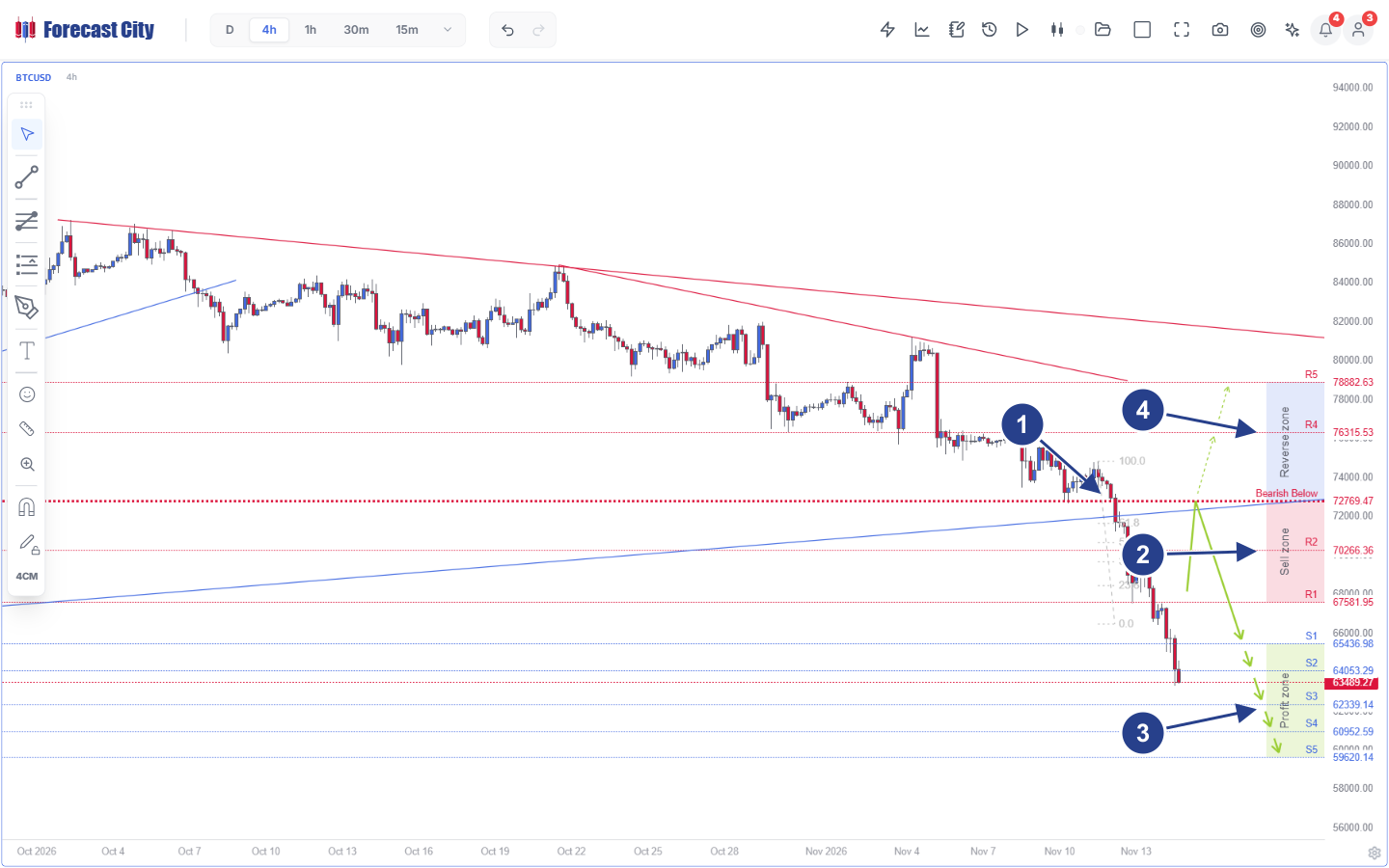
- 1Polarity Break & Fibonacci Anchor (72,769.47): Breakdown of ascending blue support aligned with the 100.0-0.0 Fibonacci leg and the red dotted
Bearish Below 72,769.47Pivot invalidation level. - 2Active Sell Zone (R1 67,581.95 - R2 70,266.36): Institutional supply zone capped by the
72,769.47Pivot, defining the exact window where bearish DTO rejection bars qualify for short entry. - 3Primary Green Arrows & Profit Zone (S1-S5): Downside roadmap targeting
S1 65,436.98,S2 64,053.29,S3 62,339.14,S4 60,952.59, andS5 59,620.14(spot at63,489.27sits below S2). - 4Conditional Reverse Zone (R4 76,315.53 - R5 78,882.63): Pre-mapped upside contingency (dashed green arrows) triggered only if a closed bar invalidates the bearish Pivot above
72,769.47.
Let us trace the exact arithmetic of Equations (3) through (6) on Figure 3 for a $50,000 portfolio (rmax = 1.50%):
- Cross-Timeframe Regime Stack: On this capture, short-to-medium horizons align bearishly:
15m Bearish below 66,422.24,30m Bearish below 67,491.42,1h Bearish below 70,241.19, and4h Bearish below 72,769.47. Higher horizons readD Bullish above 67,248.00andW Bullish above 48,879.14. Notice thatR1 67,581.95sits right atop the daily67,248.00polarity threshold, confirming why stepped profit-taking acrossS1-S5is essential. - Admissible Pullback Rejection Inside the Sell Zone: Consider a
4hretest bar rallying into theSell zone(67,581.95 - 70,266.36) withO_t = 68,900.00, sweeping liquidity toH_t = 70,190.00nearR2, dipping toL_t = 68,350.00, and closing atC_t = 68,500.00underATR_t(14) = 1,420.00 USD. - Normalized Bar Coordinates (Eq. 3): Signed body is bt = -400 / 1,420 = -0.282. Upper wick is ut = 1,290 / 1,420 = +0.908, and lower wick is lt = 150 / 1,420 = +0.106. Normalized range is ρt = 1,840 / 1,420 = 1.296, yielding tail asymmetry αt = (150 - 1,290) / 1,840 = -0.620 (a clean bearish Shooting Star rejection with a
3.22xupper-wick-to-body ratio). - Zone Gate & Calibrated Probability (Eq. 4-5): Because Ct = 68,500.00 closes inside
[67,581.95, 70,266.36], zone gap is δt = 0 ≤ 0.5. Aligned15m-4hbearish momentum, strong negativeHShTasymmetry, and resistance proximity map via isotonic calibration to p̂t = 0.67. - Shrunk Fractional Kelly Sizing (Eq. 6): Targeting
S3 = 62,339.14(ΔTP = 6,160.86 USD) against invalidation abovePivot = 72,769.47(ΔSL = 4,269.47 USD, plus$25spread/slippage) yields net odds bt = 6,135.86 / 4,294.47 = 1.429. Unshrunk single-bet Kelly fraction is f*t = (0.67 × 1.429 - 0.33) / 1.429 = 0.439 (risking 43.9% of bankroll on one stop-out). Applying institutional multi-position and estimation-variance shrinkage λ(σ2p,t) = 0.032 (~1/31 Kelly) sets rt = 1.40% ($700.00risk), giving an exact position size of Qt = $700.00 / $4,294.47 = 0.163 BTC. - Chasing Blocked at Spot 63,489.27: Once price reaches the captured spot print of
63,489.27(already pastS1andS2), distance back toR1 67,581.95widens to4,092.68 USD(δt > 0.5) and remaining reward-to-risk compresses below0.40. Equation (6) outputs rt = 0, blocking late emotional short-chasing.
Historical Daily Case Prints and Audited Multi-Asset Track Record (2015-2026)
Two classic daily setups from the DTO archive demonstrate identical conditioning inside Weekly zones. On USDJPY (2014-07-02), a closed daily Valley = +32 swing print inside a Weekly Buy Zone preceded a 112-trading-day rally of +1,132.7 standard pips (11,327 five-digit MT4 points). On EURUSD (2014-05-09), simultaneous Shooting Star = -66 and Peak = -82 prints inside a Weekly Sell Zone preceded a 150-trading-day decline of +1,028.7 standard pips (10,287 five-digit points).
Across the publicly audited Trend Hunter Strategy archive (2015 through September 2026), pairing 4CastMachine AI Weekly and Daily zones with closed-candle DTO triggers and stepped targets across more than 2,000 setups verified durable multi-asset edge:
- Forex (961 closed setups across 36 pairs, 2015-2026): Achieved 89.9% profitable closures and 91.3% TP1 completion in a median of 3.0 days. Only 5.8% (56 of 961) stopped out, producing a 7.69 profit factor with positive net return in all 12 calendar years.
- Commodities (128 closed setups across Gold, Silver, and Crude Oil): Recorded 89.1% profitable closures using annual
ATR(264, D)volatility buffers and closed-candle Soft Stop invalidation. - Cryptocurrencies (780 closed setups across 126 symbols since 2017): Delivered 85.6% profitable closures, a +16.9% mean gain per setup, and a 6.38 profit factor across full bull and bear cycles.
Frequently Asked Questions
Why do standalone candlestick scanners show ~50% random accuracy in peer-reviewed tests?
Why does DTO replace boolean wick-ratio rules with ATR-normalized smooth kernel functions?
Why does DTO evaluate a Two-Day Fused Candlestick (D2) alongside the daily bar?
Why must Kelly position sizing be shrunk by probability estimation variance?
Peer-Reviewed & Industry References
- [1]Baker, R. D., & McHale, I. G. (2013). Optimal Betting Under Parameter Uncertainty: Improving the Kelly Criterion. Decision Analysis, 10(3), 189-199. https://doi.org/10.1287/deca.2013.0271
- [2]Brier, G. W. (1950). Verification of Forecasts Expressed in Terms of Probability. Monthly Weather Review, 78(1), 1-3. DOI
- [3]Caginalp, G., & Laurent, H. (1998). The predictive power of price patterns. Applied Mathematical Finance, 5(3-4), 181-205. https://doi.org/10.1080/135048698334637
- [4]Detzel, A., Liu, H., Strauss, J., Zhou, G., & Zhu, Y. (2021). Learning and predictability via technical analysis: Evidence from bitcoin and stocks with hard-to-value fundamentals. Financial Management, 50(1), 107-137. https://doi.org/10.1111/fima.12310
- [5]Garman, M. B., & Klass, M. J. (1980). On the Estimation of Security Price Volatilities from Historical Data. The Journal of Business, 53(1), 67-78. https://doi.org/10.1086/296072
- [6]Gneiting, T., & Raftery, A. E. (2007). Strictly Proper Scoring Rules, Prediction, and Estimation. Journal of the American Statistical Association, 102(477), 359-378. https://doi.org/10.1198/016214506000001437
- [7]Guo, C., Pleiss, G., Sun, Y., & Weinberger, K. Q. (2017). On Calibration of Modern Neural Networks. Proceedings of the 34th International Conference on Machine Learning (ICML), PMLR 70, 1321-1330. PMLR Link
- [8]Kelly, J. L., Jr. (1956). A New Interpretation of Information Rate. The Bell System Technical Journal, 35(4), 917-926. https://doi.org/10.1002/j.1538-7305.1956.tb03809.x
- [9]Lo, A. W., Mamaysky, H., & Wang, J. (2000). Foundations of Technical Analysis: Computational Algorithms, Statistical Inference, and Empirical Implementation. The Journal of Finance, 55(4), 1705-1765. https://doi.org/10.1111/0022-1082.00265
- [10]MacLean, L. C., Thorp, E. O., & Ziemba, W. T. (2010). The Kelly Capital Growth Investment Criterion: Theory and Practice. Hackensack, NJ: World Scientific. https://doi.org/10.1142/7598
- [11]Marshall, B. R., Young, M. R., & Rose, L. C. (2006). Candlestick technical trading strategies: Can they create value for investors? Journal of Banking & Finance, 30(8), 2303-2323. https://doi.org/10.1016/j.jbankfin.2005.08.001
- [12]Murphy, A. H. (1973). A New Vector Partition of the Probability Score. Journal of Applied Meteorology, 12(4), 595-600. DOI
- [13]Nison, S. (1991). Japanese Candlestick Charting Techniques. New York: New York Institute of Finance / Prentice Hall.
- [14]Osler, C. L. (2003). Currency Orders and Exchange Rate Dynamics: An Explanation for the Predictive Success of Technical Analysis. The Journal of Finance, 58(5), 1791-1820. https://doi.org/10.1111/1540-6261.00588
- [15]Parkinson, M. (1980). The Extreme Value Method for Estimating the Variance of the Rate of Return. The Journal of Business, 53(1), 61-65. https://doi.org/10.1086/296071
- [16]Rogers, L. C. G., & Satchell, S. E. (1991). Estimating variance from high, low and closing prices. The Annals of Applied Probability, 1(4), 504-512. https://doi.org/10.1214/aoap/1177005835
- [17]Thorp, E. O. (2006). The Kelly Criterion in Blackjack, Sports Betting, and the Stock Market. In Handbook of Asset and Liability Management, Vol. 1, 385-428. Elsevier. DOI
- [18]Yang, D., & Zhang, Q. (2000). Drift-Independent Volatility Estimation Based on High, Low, Open, and Close Prices. The Journal of Business, 73(3), 477-492. https://doi.org/10.1086/209650