Commercial black-box trading bots and opaque buy/sell alert feeds routinely advertise annualized Sharpe ratios above 2.0 in historical backtests yet collapse once live capital is deployed. We establish the root causes of this failure across three rigorous dimensions. First, unconstrained hyperparameter search across finite price histories converts Gaussian noise into illusory alpha, quantified via the Deflated Sharpe Ratio (DSR) and Combinatorially Symmetric Cross-Validation Probability of Backtest Overfitting (PBO). Second, post-hoc feature-attribution wrappers (LIME and SHAP) evaluate correlated financial features off the true regime manifold and exhibit severe tick-by-tick Lipschitz instability without specifying price-space risk coordinates. Third, scalar point-arrow outputs leave human operators blind during Maximum Adverse Excursion (MAE) drawdowns, inducing premature panic exits or unhedged catastrophic holding. We contrast opaque bots against the glass-box prescriptive geometry of 4CastMachine AI, walking step by step through live XAUUSD Daily and GBPUSD 4h roadmaps and closing the behavioral execution loop through AI Strategy Studio, Virtual Accounts, and AI Trading Journal.
1. Multiple-Testing Selection Bias: Deflated Sharpe Ratio and Backtest Overfitting
Walk through the standard engineering pipeline behind a commercial black-box trading bot. Because the model contains no structural prior anchored in market microstructure or order-book geometry, its developers sweep thousands of neural network checkpoints, lookback windows, stop distances, and entry thresholds across a fixed historical price sample of length T. At the end of that sweep, only the single highest-scoring configuration n* = arg maxn∈{1..N} SR̂n appears on the marketing page.
Bailey, Borwein, López de Prado, and Zhu [12, 14] proved that this unconstrained search pipeline turns ordinary random variance into persuasive historical equity curves. Even if every single candidate bot in a pool of N strategies has zero true forward edge (SRn = 0 for all n), taking the maximum across N noisy trials shifts the expected winner far into the right tail of the Gaussian distribution.
Using Extreme Value Theory for the maximum of N independent trials with cross-trial Sharpe variance V[{SR̂n}], Bailey and López de Prado [13] derived the expected false-positive maximum Sharpe ratio SR0(N) under the pure-noise null hypothesis:
Every symbol in Equation (1) has a direct statistical meaning. The factor √(V[{SR̂n}]) is the cross-sectional standard deviation of realized Sharpe ratios across the N tested parameter sets. The constant γEM ≈ 0.5772 is the Euler-Mascheroni constant governing Gumbel extreme-value convergence, e ≈ 2.7183 is Euler's number, and Φ-1(·) is the inverse standard normal cumulative distribution function.
Flipping a fair coin ten times rarely yields ten heads, yet asking 2,500 people to flip ten coins almost guarantees that somebody will boast a "perfect coin-flipping algorithm." Equation (1) computes the exact Sharpe hurdle SR0(N) you should expect from pure luck alone when a developer tests N black-box variations on historical candles.
Financial return series add a second trap on top of trial multiplicity: strategies that sell tail convexity or hold losing positions exhibit negative skewness (γ̂3 < 0) and fat-tailed kurtosis (γ̂4 > 3), both of which inflate the standard error of an estimated Sharpe ratio. Incorporating sample length T and higher return moments yields the Deflated Sharpe Ratio (DSR, Bailey and López de Prado [13]):
In Equation (2), SR̂n* is the non-annualized in-sample Sharpe ratio of the selected winner over T observations, SR0(N) is the multiple-testing hurdle from Equation (1) in matching units, γ̂3 is sample skewness, γ̂4 is sample kurtosis (where a normal distribution equals 3.0), and Φ(·) converts the deflated z-statistic into a probability in (0, 1).
A reported Sharpe ratio is meaningless until you subtract the luck hurdle SR0(N) in the numerator and penalize crash-prone negative skew and fat tails in the denominator. Whenever SR̂n* sits below SR0(N), DSR drops below 0.50, proving that the dazzling backtest is statistically indistinguishable from data-mined noise.
Work through a realistic vendor audit step by step. Suppose a bot developer sweeps N = 2,500 neural and indicator configurations over T = 500 daily bars (two trading years), observing annualized cross-trial Sharpe dispersion √V = 0.65. First evaluate the two normal quantiles in Equation (1): Φ-1(1 - 1/2500) = Φ-1(0.9996) = 3.3528, and Φ-1(1 - 1/(2500 × e)) = Φ-1(0.999853) = 3.6205. Weighting by (1 - 0.5772) and 0.5772 produces bracket factor 0.4228(3.3528) + 0.5772(3.6205) = 3.5073. Multiplying by 0.65 yields an annualized noise hurdle of SR0(2500) = 2.280 (or 2.280 / √252 = 0.1436 per daily bar).
Now suppose the vendor markets the winning bot with an advertised annualized Sharpe of 2.05 (SR̂n* = 0.1291 daily), sample skewness γ̂3 = -0.85, and fat kurtosis γ̂4 = 6.50. Plugging into Equation (2), the numerator is (0.1291 - 0.1436) × √499 = -0.3239, while the denominator is √(1 - (-0.85)(0.1291) + (5.50/4)(0.1291)2) = 1.0643. The resulting statistic is DSR = Φ(-0.304) = 0.381, failing a standard 95% confidence hurdle (0.95) by a wide margin. Bailey et al. [14] confirmed this result via Combinatorially Symmetric Cross-Validation (CSCV). Across unconstrained parameter grids, the Probability of Backtest Overfitting (PBO) routinely exceeded 0.75, meaning three out of four in-sample winners underperformed the median strategy out of sample.
2. Why Post-Hoc Feature Attribution (LIME and SHAP) Cannot Rescue Black Boxes
Aware that institutional and experienced retail traders distrust naked buy/sell arrows, several quantitative vendors bolt post-hoc explainability panels onto their black-box classifiers using LIME (Ribeiro, Singh, and Guestrin [2]) or SHAP (Lundberg and Lee [3]). Rudin [1] articulated the fundamental flaw of this patch in high-stakes decision making: a post-hoc explanation model is a separate approximation that cannot be globally faithful to the underlying black box without replacing it outright.
When applied to non-stationary financial time series, perturbation-based feature attribution breaks down mathematically. Both LIME and interventional KernelSHAP estimate the importance of feature subset S at current market state xt ∈ ℝp by splicing current values xt,S with background values X-S drawn from historical marginal data, while attribution stability is governed by the local Lipschitz constant (Alvarez-Melis and Jaakkola [4]):
In Equation (3), f(·) is the opaque classifier score, xt,S holds the active feature subset fixed at timestamp t, and dℙ(x-S) integrates remaining features over their unconditional historical marginal distribution rather than their regime-conditional distribution dℙ(x-S | xt,S, Rt). On the right, ϕ(f, xt) is the resulting attribution vector and δ is a tiny market perturbation inside ball radius r.
Equation (3) exposes two fatal flaws of SHAP/LIME bars on trading screens. First, splicing today's panic-level 5-minute volatility with last summer's sleepy 4-hour spread evaluates the neural network on synthetic "Frankenstein" market states that never occur in nature. Second, because Lϕ(xt) ≫ 1 near steep nonlinear decision boundaries, a routine half-pip bid-ask bounce δ can flip the top explanation bar from "RSI drove this buy" to "volume drove this buy" on the very next tick.
Even more importantly, Kumar et al. [6] and Slack et al. [5] showed that post-hoc attributions answer the wrong operational question. Consider a concrete numerical readout: suppose a deep-learning bot flashes BUY EURUSD @ 1.0880 alongside a SHAP bar stating 4h_realized_vol = +0.21 log-odds, 15m_order_imbalance = +0.14 log-odds. Two minutes later, a 0.7-pip quote flicker (‖δ‖2 = 0.012) shifts the attribution vector by ‖Δϕ‖2 = 0.29, yielding local sensitivity Lϕ = 24.2. Worse still, neither vector exists in price-time coordinates ℝ+ × [t0, ∞). Feature-importance bars never tell the trader what price band offers positive reward-to-risk entry, what exact chart price proves the thesis wrong, or where partial profits belong.
3. Sequential Ambiguity Under Adverse Excursion vs. Glass-Box Stopping-Time Geometry
The deepest failure of black-box bots unfolds after real money enters the market. Almost every winning trade experiences temporary adverse movement before reaching its target. Sweeney [15] formalized this pathwise drawdown as Maximum Adverse Excursion (MAE): for a long position opened at price Pt_0, MAEt_0,t = maxu∈[t_0,t](Pt_0 - Pu)+ = d > 0.
Suppose a trader follows an opaque bot output ât_0 = +1 (BUY @ P_0) and price immediately pulls back by d = 24 pips while the bot stays silent or repeats +1. Because the bot hides its internal validity region, the human operator faces an unidentifiable sequential hypothesis test at every losing tick: is drawdown d ordinary diffusive order-book noise inside a healthy setup (ℋ0), or has the market shifted into a structural breakdown outside the bot's training distribution (ℋ1)?
Clinical physiological studies of live day-traders by Lo, Repin, and Steenbarger [9] and bank dealers by Fenton-O'Creevy et al. [10] show why this ambiguity is destructive. Floating loss without an observable invalidation boundary spikes autonomic arousal and triggers two opposite wealth-destroying behaviors. Many operators panic, close manually near the bottom of ordinary ℋ0 noise, and fall into algorithm aversion by abandoning the model right before its recovery winners (Dietvorst, Simmons, and Massey [7]). Other operators freeze during genuine ℋ1 regime failure and hold unhedged drawdowns until margin liquidation (Apesteguia, Oechssler, and Weidenholzer [11]).
Figure 1 contrasts this unidentifiable black-box drawdown trap against the observable price-space geometry of a 4CastMachine AI glass-box roadmap.
Mathematically, 4CastMachine AI replaces opaque scalar alerts with an inherently interpretable geometric specification in price-time coordinates. Extending López de Prado's [15] Triple-Barrier concept into a complete dual-scenario roadmap, every active forecast on symbol s and timeframe τ projects an explicit tuple and first-passage stopping-time pair:
At forecast generation timestamp t0, Navigator AI projects onto price space ℝ+ the structural roadmap tuple:
For a bullish roadmap (Ppivot labeled Bullish Above), trade execution and thesis invalidation are governed by observable first-passage stopping times:
Here 𝒵entry is the shaded Buy Zone (or Sell Zone), 𝒞τ(t) ∈ {0, 1} is the closed-candlestick rejection confirmation indicator on timeframe τ, Ppivot is the exact structural invalidation price, {TPk}k=1K are stepped Profit Zone targets, γmain denotes primary solid Green Arrows, and γalt denotes conditional Dashed Arrows inside Reverse Zone 𝒵rev (with intraday volatility buffer βτ = 0.10 on 5m-4h or closed Daily candle confirmation on D).
Equations (4) and (5) bring Karl Popper's scientific criterion of falsifiability directly onto the trading screen. Before a single dollar is risked, you know the exact zone where buyers or sellers should defend structure (𝒵entry), the closed candle required to prove they showed up (𝒞τ = 1), and the exact price (Ppivot) that falsifies the thesis. As long as price remains on the valid side of Ppivot, floating MAE is objectively classified as ℋ0 noise.
Check the risk symmetry numerically. Suppose a bullish 1h setup prints Buy Zone = 1.08500-1.08640 and Bullish Above 1.08500 (Ppivot = 1.08500) with annual daily true range ATR(264, D) = 68 pips and live spread 0.8 pips. By Equation (5), the intraday protective stop sits at 1.08500 - 0.10(0.00680) - 0.00008 = 1.08424. If a closed 1h rejection candle confirms at 1.08564, total falsification risk is fixed at exactly 14.0 pips (1.0R). Any pullback to 1.08520 (-4.4 pips MAE) remains 2.0 pips above Ppivot and 9.6 pips above τinv, removing emotional guesswork completely.
4. Live Glass-Box Anatomy Across Horizons: XAUUSD Daily and GBPUSD 4h
Inspecting live charts on 4CM-AI Charts shows how Definition 1 adapts cleanly across both Daily macro horizons and 4-hour intraday horizons, while keeping every historical cycle permanently visible for audit.
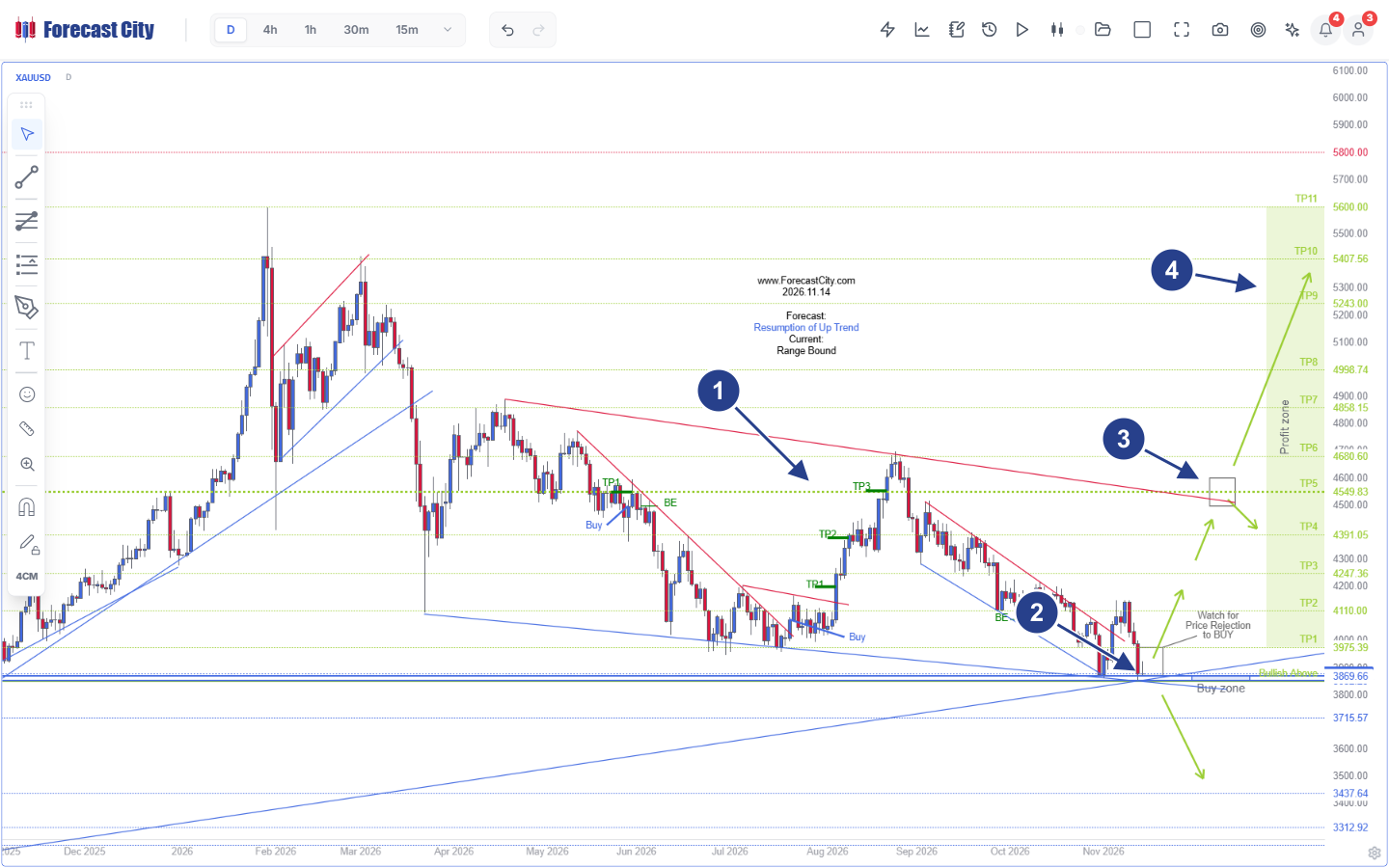
- 1Converging Wedge & Audited Past Cycles: Multi-month descending red resistance and ascending blue support frame permanently stamped prior setups (
May/Jun Buy -> TP1 -> BE,Aug Buy -> TP1 -> TP2 -> TP3, andOct BE). - 2Buy Zone & Bullish Above 3869.66 Floor: Under
Forecast: Resumption of Up Trend | Current: Range Bound, price tests the structuralBuy zoneanchored atBullish Above 3869.66(backed by3715.57and3437.64). - 3Rejection Prompt & TP5 Decision Fork: Chart specifies
Watch for Price Rejection to BUYat entry and draws an explicit decision node box at the upper red wedge line (TP5 4549.83) showing rejection vs. breakout paths. - 4Stepped Profit Zone Ladder (TP1-TP11): Primary solid green trajectory maps sequential targets
TP1 3975.39,TP2 4110.00,TP3 4247.36,TP4 4391.05, andTP5 4549.83up toTP11 5600.00.
Examine Figure 2 (XAUUSD D) carefully from left to right. Unlike commercial alert channels that quietly delete losing setups or overwrite past arrows, 4CM-AI Charts stamps historical trade lifecycles directly onto the price history (marker 1). You can verify May/June's Buy reaching TP1 before closing the runner at Break-Even (BE), August's wedge bounce advancing sequentially through TP1, TP2, and TP3 right at upper red trendline resistance, and October's BE protection. At the current right edge (marker 2), Gold sits inside the Buy zone right above Bullish Above 3869.66 with explicit instruction Watch for Price Rejection to BUY. Notice also marker 3: rather than pretending resistance does not exist, Navigator AI places a rectangular decision node right where TP5 4549.83 intersects the multi-month descending red trendline, mapping both a tactical pullback toward TP4 4391.05 and the continuation leg toward TP6 4680.60 through TP11 5600.00 (marker 4).
Now compare that Daily macro roadmap against an active intraday 4h roadmap on British Pound / US Dollar (GBPUSD 4h) in Figure 3.
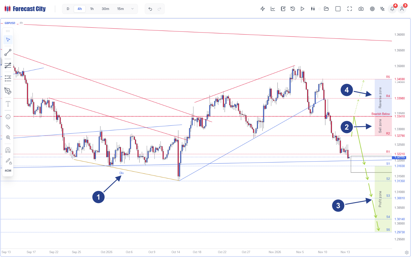
- 1Bullish Divergence & Broken Channel: Prior gold
Divtrendline (Sep 25 to Oct 15) launched an ascending blue channel that broke downward in mid-November, leaving spot at1.32115. - 2Sell Zone & Bearish Below 1.33410 Pivot: Overhead supply spans
R1 1.32210and shadedSell zoneR2 1.32790up to the dotted red invalidation boundaryBearish Below 1.33410. - 3Primary Green Arrows & Profit Zone: Solid green arrows project continuation from the
Sell zonethrough theS1consolidation box intoS1 1.31830,S2 1.31350,S3 1.30810,S4 1.30140, andS5 1.29730. - 4Conditional Reverse Zone (Dashed Arrows): Above
1.33410, the shaded blueReverse zonemaps upside contingency targetsR4 1.33980andR5 1.34590via dashed green arrows if a 4h candle closes above the Pivot.
Comparing Figure 2 (XAUUSD D) and Figure 3 (GBPUSD 4h) highlights an intentional, microstructure-grounded design distinction across timeframes. Why does the Daily chart in Figure 2 render primary solid Green Arrows (with structural fork branches at trendline boundaries), whereas the 4h chart in Figure 3 renders both primary solid Green Arrows toward the Profit zone (S1 1.31830 down to S5 1.29730) and conditional Dashed Arrows inside a shaded Reverse zone (R4 1.33980 to R5 1.34590)?
The answer lies in horizon execution physics. On the D (Daily) timeframe, multi-week institutional positioning follows ForecastCity's Soft Stop Loss rule. An intraday wick across 3869.66 during New York volatility does not invalidate a multi-month wedge floor unless a full Daily candle closes decisively beyond support. Macro roadmaps therefore emphasize primary structural legs and trendline decision forks rather than instant intraday flip-and-reverse trades. On 4h and lower intraday timeframes (5m through 4h), tight stop clusters sit directly behind key pivots such as Bearish Below 1.33410. When institutional flow forces a closed 4h candle above 1.33410, short-covering fuels an immediate impulse across the Reverse zone toward R4 1.33980 and R5 1.34590. Pre-drawing those conditional Dashed Arrows before entry eliminates post-stop hesitation.
| Decision Dimension | Opaque Black-Box Bots & Alert Channels | Black-Box Classifier + SHAP / LIME | 4CastMachine AI Prescriptive Chart Roadmap |
|---|---|---|---|
| Primary Output Space | Scalar command (BUY / SELL NOW) with hidden internal state. |
Scalar score plus abstract feature-weight bar chart. | Price-time geometry: Buy/Sell Zone, Pivot, TP1-TP5 Profit Zone, Reverse Zone, Green & Dashed Arrows. |
| Entry Execution Discipline | Chases post-impulse market orders or sets blind limit traps. | No structural entry band; reacts bar-by-bar to feature drift. | Conditional stopping time τentry: waits for zone test plus closed candlestick confirmation. |
| Epistemic Falsifiability | Unfalsifiable during MAE drawdown; arbitrary fixed-pip stops. | Attributions shift tick-by-tick without defining invalidation price. | Explicit Pivot boundary Ppivot: buffered by 10% ATR(264, D) intraday or closed-candle Soft Stop on D. |
| Contingency on Breakdown | Silent failure or lagging flip after drawdown completes. | Recomputes post-hoc weights only after loss occurs. | Pre-mapped alternate path γalt: Dashed Arrows across Reverse Zone (5m-4h) eliminate post-loss freeze. |
| Human Agency & Auditability | Take-it-or-leave-it lock (32% retention after error; Dietvorst [8]). | Read-only inspection; cannot modify or replay strategy rules. | Modifiable co-pilot (68%-76% retention [8]): rule calibration in AI Strategy Studio + Shadow Variant audit. |
5. Modifiable Human Agency, GBPUSD 4h Micro-Anatomy, and Shadow Variant Auditing
Why does glass-box modifiability matter quantitatively? Dietvorst, Simmons, and Massey [8] proved in controlled incentive-compatible experiments that when operators are locked out of an imperfect forecasting model ("take it or leave it"), only 32% continue using it after observing normal forecast errors. When operators can inspect the model's structure and adjust bounded execution parameters, sustained adoption rises to 68%-76% and realized portfolio performance improves substantially. ForecastCity, the all-in-one AI platform for traders, operationalizes this modifiable workflow across four integrated surfaces.
Trace two operators trading the exact GBPUSD 4h structure shown in Figure 3 on a $10,000 account with a 1.0% ($100) risk budget and annual daily true range ATR(264, D) = 82 pips.
Opaque Bot Operator: Receives a naked momentum alert SELL GBPUSD @ 1.32120 right at the bottom of the breakdown candle near S1 consolidation. Over the next two 4h bars, routine institutional profit-taking retraces GBPUSD upward by 64 pips to 1.32760. Staring at an unanchored floating drawdown with zero chart invalidation line, the operator panics, closes manually at 1.32755 for a realized -$127 loss, and disables the bot minutes before sellers step into the institutional Sell zone.
Glass-Box Operator: Sets an alert on the Figure 3 roadmap (Sell zone R2 1.32790 up to Bearish Below 1.33410) and waits patiently while price is still down at 1.32115. When GBPUSD rallies into the Sell zone and closes a 4h Bearish Rejection candle at 1.32820, AI Strategy Studio computes the structural stop above 1.33410 plus 10% ATR(264, D) (8.2 pips) and 0.9 pip spread: Pstop = 1.33501. Exact stop distance is 68.1 pips, sizing the trade at 0.15 standard lots ($102 = 1.0R). Any intra-zone wick to 1.33180 remains 23 pips below Pivot 1.33410, confirming ℋ0 calmly. Reaching S1 = 1.31830 (+99.0 pips, +1.45R) banks partial profit and moves the remaining stop to Break-Even (1.32810), eliminating downside tail risk while runners target S2 = 1.31350 (+2.16R) and S3 = 1.30810 (+2.95R).
Before committing live capital, traders verify their four explicit strategy clauses (Entry, Stop Loss, Take Profit, and Management) on historical candles inside AI Strategy Studio's Test tab with realistic spread and commission friction. Next, they forward-test on live streaming ticks inside Virtual Accounts, where optional public track records are cryptographically sealed by a tamper-evident SHA-256 hash chain so losing trades can never be hidden retroactively.
Even with a transparent chart roadmap, human operators still occasionally hesitate on entries, widen stops, or cut winners early. To separate model edge from human execution drift, ForecastCity simulates an untouched zero-override Shadow Variant alongside every Virtual Account or ForecastFollow (MetaTrader 4/5) trade. Inside AI Trading Journal, the Strategy check engine decomposes net behavioral P&L divergence across five orthogonal execution clauses:
In Equation (6), P&Lrealized is actual account net profit over a review window, P&Lshadow is the exact counterfactual profit generated by the trader's saved rules with zero manual overrides, and each δm isolates currency impact attributable to clause m.
When an opaque bot loses money, nobody knows whether the model broke or the human interfered at the worst moment. Equation (6) acts like a flight-data recorder for trading discipline: it measures to the exact dollar how much every manual early exit, skipped confirmation, or moved stop helped or hurt your bottom line relative to your own baseline plan.
Consider a concrete 30-trade monthly audit in AI Trading Journal. Suppose the untouched Shadow Variant earned P&Lshadow = +$1,180, whereas the human operator finished at P&Lrealized = +$760 (ΔP&Lhuman = -$420). Equation (6) breaks that -$420 gap into actionable clauses: disciplined zone entries added δEntry = +$35, unchanged position sizing gave δRisk = $0, dragging stops twice cost δSL = -$145, skipping Break-Even shifts cost δMgmt = -$65, and closing winners manually ahead of TP2 cost δTP = -$245. Instead of discarding a sound analytical engine out of frustration, the trader sees the exact behavioral leak (premature profit-taking) and corrects it objectively.
Frequently Asked Questions
Why do high-Sharpe backtested trading bots so often lose money in live markets?
Why are SHAP or LIME feature bars insufficient for live capital risk management?
How does the Pivot level eliminate emotional panic during normal trade pullbacks?
Why do 4h roadmaps show Dashed Arrows in a Reverse Zone while Daily roadmaps show solid Green Arrows?
How do Shadow Variants and Strategy Check measure human interference?
Peer-Reviewed & Industry References
- [1]Rudin, C. (2019). Stop Explaining Black Box Machine Learning Models for High Stakes Decisions and Use Interpretable Models Instead. Nature Machine Intelligence, 1(5), 206-215. https://doi.org/10.1038/s42256-019-0048-x
- [2]Ribeiro, M. T., Singh, S., & Guestrin, C. (2016). "Why Should I Trust You?": Explaining the Predictions of Any Classifier. Proceedings of the 22nd ACM SIGKDD International Conference on Knowledge Discovery and Data Mining, 1135-1144. https://doi.org/10.1145/2939672.2939778
- [3]Lundberg, S. M., & Lee, S.-I. (2017). A Unified Approach to Interpreting Model Predictions. Advances in Neural Information Processing Systems 30 (NeurIPS 2017), 4765-4774. arXiv:1705.07874
- [4]Alvarez-Melis, D., & Jaakkola, T. S. (2018). On the Robustness of Interpretability Methods. ICML WHI 2018, https://doi.org/10.48550/arXiv.1806.08049
- [5]Slack, D., Hilgard, S., Jia, E., Singh, S., & Lakkaraju, H. (2020). Fooling LIME and SHAP: Adversarial Attacks on Post hoc Explanation Methods. Proceedings of the AAAI/ACM Conference on AI, Ethics, and Society (AIES 2020), 180-186. https://doi.org/10.1145/3375627.3375830
- [6]Kumar, I. E., Venkatasubramanian, S., Scheidegger, C., & Friedler, S. A. (2020). Problems with Shapley-Value-Based Explanations as Feature Importance Measures. Proceedings of the 37th International Conference on Machine Learning (ICML 2020), PMLR 119, 5491-5500. arXiv:2002.11097
- [7]Dietvorst, B. J., Simmons, J. P., & Massey, C. (2015). Algorithm Aversion: People Erroneously Avoid Algorithms After Seeing Them Err. Journal of Experimental Psychology: General, 144(1), 114-126. https://doi.org/10.1037/xge0000033
- [8]Dietvorst, B. J., Simmons, J. P., & Massey, C. (2018). Overcoming Algorithm Aversion: People Will Use Imperfect Algorithms If They Can (Even Slightly) Modify Them. Management Science, 64(3), 1155-1170. https://doi.org/10.1287/mnsc.2016.2643
- [9]Lo, A. W., Repin, D. V., & Steenbarger, B. N. (2005). Fear and Greed in Financial Markets: A Clinical Study of Day-Traders. American Economic Review, 95(2), 352-359. https://doi.org/10.1257/000282805774670095
- [10]Fenton-O'Creevy, M., Soane, E., Nicholson, N., & Willman, P. (2011). Thinking, Feeling and Deciding: The Influence of Emotions on the Decision Making and Performance of Traders. Journal of Organizational Behavior, 32(8), 1044-1061. https://doi.org/10.1002/job.720
- [11]Apesteguia, J., Oechssler, J., & Weidenholzer, S. (2020). Copy Trading. Management Science, 66(12), 5608-5622. https://doi.org/10.1287/mnsc.2019.3508
- [12]Bailey, D. H., Borwein, J. M., López de Prado, M., & Zhu, Q. J. (2014). Pseudo-Mathematics and Financial Charlatanism: The Effects of Backtest Overfitting on Out-of-Sample Performance. Notices of the American Mathematical Society, 61(5), 458-471. https://doi.org/10.1090/noti1105
- [13]Bailey, D. H., & López de Prado, M. (2014). The Deflated Sharpe Ratio: Correcting for Selection Bias, Backtest Overfitting, and Non-Normality. The Journal of Portfolio Management, 40(5), 94-107. https://doi.org/10.3905/jpm.2014.40.5.094
- [14]Bailey, D. H., Borwein, J. M., López de Prado, M., & Zhu, Q. J. (2017). The Probability of Backtest Overfitting. The Journal of Computational Finance, 20(4), 39-69. https://doi.org/10.21314/JCF.2016.322
- [15]López de Prado, M. (2018). Advances in Financial Machine Learning. Hoboken, NJ: John Wiley & Sons (Ch. 3, Triple-Barrier Method); & Sweeney, J. (1997). Maximum Adverse Excursion: Analyzing Price Fluctuations for Trading Management. New York: John Wiley & Sons.