Classical retail and institutional charting workspaces pass non-stationary price series through causal trailing filters such as Simple Moving Averages (SMA), Exponential Moving Averages (EMA), MACD, RSI, Stochastic oscillators, and Bollinger Bands. Using Discrete-Time Fourier Transform group-delay derivations, Roy-Vetterli spectral effective rank, and multiple-hypothesis False Discovery Rate (FDR) bounds, this paper demonstrates why descriptive indicator stacks systematically induce analysis paralysis. Across empirical foreign exchange, precious metal, and cryptocurrency series, ten-indicator momentum workspaces collapse to an effective dimensionality between 1.8 and 2.6 while guaranteeing sequential sign contradictions across filter group-delay orderings whenever price tests a structural reversal zone. We then formalize how 4CastMachine AI resolves both intra-chart lag and cross-timeframe incoherence across nine horizons (1m through M) through multi-modal regime fusion, Minimum Trace (MinT) hierarchical reconciliation, and Bertsimas-Kallus conditional stochastic prescription. Live zero-indicator case studies on EURUSD D and ETHUSD 4h inside 4CM-AI Charts illustrate how Navigator AI renders one falsifiable flight plan while preserving human supervisory authority.
1. Causal Phase Lag and Group Delay in Classical Trailing Indicators
Open almost any discretionary chart after a sharp trend reversal and a familiar timing failure appears. Price tests a multi-week institutional support shelf, prints an impulsive rejection candle, and rallies forty percent of its eventual swing range while the moving averages and momentum sub-panes below the chart still point downward. Only after the bulk of the asymmetric reward-to-risk move has already elapsed do the trailing lines finally cross upward, inviting late entries right into short-term exhaustion.
That timing failure is not an accidental flaw of poor parameter tuning. It is an inescapable mathematical consequence of applying causal discrete-time filters to non-stationary financial price series. At bar index t, future closes Pt+1, Pt+2, ... have not yet occurred. Any indicator computed solely from historical bar closes {Pt-k}k≥0 must obey the causality constraint h[k] = 0 for all k < 0, where h[k] denotes the filter impulse response.
Under the Discrete-Time Fourier Transform (Oppenheim and Schafer [8]), a linear time-invariant filter maps an input sinusoid at normalized angular frequency ω ∈ (-π, π] (measured in radians per bar) through the complex frequency response H(ejω) = |H(ejω)| ejϕ(ω). Here |H(ejω)| is the magnitude gain that attenuates high-frequency chop, and ϕ(ω) is the continuous phase shift. When a localized price wave packet or trend inflection centered near frequency ω passes through the filter, its envelope is delayed in time by a precise number of bars known as the group delay τg(ω) = -dϕ(ω) / dω. Evaluating this transfer function for an N-bar Simple Moving Average (h[k] = 1/N for 0 ≤ k ≤ N - 1) yields our first structural constraint:
Every term in Equation (1) carries a direct operational consequence on a live trading screen. The integer N is the lookback window length in bars, the Dirichlet ratio sin(ωN / 2) / [N sin(ω / 2)] governs amplitude smoothing, and the linear phase factor e-jω(N - 1)/2 differentiates to a constant group delay of exactly (N - 1) / 2 bars across every frequency ω.
An equal-weighted moving average computes the center of mass of the most recent N closes. The temporal midpoint of a window spanning bar t - (N - 1) through bar t sits exactly (N - 1) / 2 bars in the past. Worse still, chopping history abruptly at bar t - N multiplies price by a rectangular boxcar window, whose Fourier transform exhibits -13.3 dB spectral sidelobes (Gibbs ringing). When a central-bank rate decision creates a single large jump candle, an SMA echoes a phantom counter-move N bars later purely when that old candle drops out of the trailing window.
Consider a concrete numerical calculation on a 4h foreign-exchange or cryptocurrency chart. An SMA(20) imposes a group delay of (20 - 1) / 2 = 9.5 bars, which equals 38 hours of real market elapsed time. An SMA(50) lags by (50 - 1) / 2 = 24.5 bars, or 98 hours (more than four full trading days). A benchmark SMA(200) lags structural regime shifts by 99.5 bars, or 398 hours (over three FX trading weeks). If EURUSD reverses from an institutional support zone and completes a 180-pip impulse over forty hours, an SMA(20) / SMA(50) crossover literally cannot confirm the turn until more than half the move is already behind the trader.
Aware of boxcar lag, practitioners routinely switch from Finite Impulse Response (FIR) moving averages to recursive Infinite Impulse Response (IIR) filters such as the Exponential Moving Average, defined by yt = α Pt + (1 - α) yt-1 with smoothing factor α = 2 / (N + 1). Taking the z-transform HEMA(z) = α / [1 - (1 - α)z-1] and differentiating its unwrapped phase with respect to ω reveals why exponential weighting never escapes the causal barrier:
In Equation (2), α ∈ (0, 1) is the weight placed on the current close Pt, while (1 - α) governs exponential memory decay across all prior closes. Evaluating τg,EMA(ω) as ω → 0 (the low-frequency band that carries sustained directional trends) collapses the fraction cleanly to (1 - α) / α, which under standard parameterization α = 2 / (N + 1) equals the exact same (N - 1) / 2 bar delay as an SMA(N).
Replacing an SMA(N) with an EMA(N) eliminates drop-off echoes, yet preserves the full (N - 1) / 2 bar delay on underlying trends while introducing nonlinear phase distortion: fast high-frequency jiggles pass through with tiny delay, whereas persistent low-frequency waves lag far behind, warping waveform geometry. By Bode's gain-phase integral relation (Ehlers [3]; Oppenheim and Schafer [8]), no causal filter operating solely on past prices can simultaneously reject high-frequency noise and achieve zero phase delay.
Cascaded oscillators compound this delay further. An EMA(20) (α = 2/21 ≈ 0.0952) carries 9.5 bars of low-frequency trend lag. Wilder's classic RSI(14) smooths upward and downward bar increments using recursive weight α = 1/14 ≈ 0.0714; solving (1 - α) / α = 13 / 1 shows that RSI(14) embeds the exact low-frequency group delay of an EMA(27), or 13.0 bars. Similarly, MACD(12, 26, 9) subtracts a 12.5-bar-lagging EMA(26) from a 5.5-bar-lagging EMA(12) and then passes that difference through a third 9-bar EMA trigger stage, adding 4.0 extra bars of smoothing delay right when momentum inflects. Every descriptive sub-pane reports what price already did several bars ago, never where institutional order books constrain future movement.
2. Multicollinearity, Effective Rank Collapse, and Real-Time Data Snooping
When a single trailing oscillator produces whipsaw losses inside choppy ranges, traders rarely question causality itself. Instead, they add a second indicator to "filter" the first, then a third to confirm the second, quickly accumulating six to ten descriptive sub-panes on one screen: RSI(14), Stochastic(14, 3, 3), CCI(20), Williams %R(14), MACD(12, 26, 9), and Bollinger %B(20). Visually, six distinct colored curves suggest six independent analytical votes.
Linear algebra exposes that independence as an illusion. Every indicator in that stack is computed from the exact same trailing window of open, high, low, and close prices. Figure 1 contrasts the signal-processing topology of a classical collinear indicator stack against the multi-modal hierarchical pipeline inside 4CastMachine AI.
To measure exactly how much independent information survives inside an M-indicator workspace, collect the standardized time series of M indicators evaluated over T bars into the matrix Z ∈ ℝT × M (with T > M, each column centered to zero mean and scaled to unit variance). Let σ1 ≥ σ2 ≥ ... ≥ σM ≥ 0 denote the singular values of Z, and define the normalized singular-value distribution pk = σk / ∑j=1M σj. Because floating-point rounding and minor nonlinearities prevent exact algebraic rank deficiency, classical integer matrix rank almost always reports rank(Z) = M even when columns are ninety percent correlated. Roy and Vetterli [11] resolved this defect by defining the continuous Effective Rank (erank) via Shannon spectral entropy:
Unpacking Equation (3), each weight pk ∈ [0, 1] measures the share of nuclear-norm amplitude carried by the k-th orthogonal principal component of the indicator panel, and H(p) is its Shannon entropy in natural logarithmic units (nats). Exponentiating H(p) maps entropy back onto the natural scale [1, M]: if all M indicators are mutually orthogonal (pk = 1/M), then H(p) = ln M and erank(Z) = M; if all M indicators are identical scalar multiples (p1 = 1, pk>1 = 0), then H(p) = 0 and erank(Z) = 1.
Expand RSI, Stochastic, CCI, Williams %R, and Bollinger %B to first order around local equilibrium price: every single one reduces to a weighted linear combination of recent bar increments ΔPt-k divided by trailing local dispersion. Consequently, over 84% of total spectral energy concentrates inside just two orthogonal modes: trailing first-difference slope (velocity) and trailing second-difference curvature (acceleration). Ten sub-panes merely redraw two lagging quantities in ten slightly rescaled coordinate systems.
Walk through a six-indicator benchmark (M = 6: RSI(14), Stochastic(14, 3), CCI(20), Williams %R(14), MACD(12, 26, 9), and Bollinger %B(20)) with singular values σ = (3.90, 1.14, 0.42, 0.24, 0.18, 0.12) and sum ∑ σj = 6.00. Spectral weights equal p = (0.650, 0.190, 0.070, 0.040, 0.030, 0.020). Summing -pk ln pk gives 1.094 nats, so erank(Z) = exp(1.094) ≈ 2.99, less than half of the six panes. Across ten-oscillator momentum templates, erank(Z) drops to 1.8 to 2.5 dimensions, creating two operational traps:
- Illusory Conviction at Trend Exhaustion: Late in an extended move, price has traveled far enough for every filter to clear its group delay τg,m. All ten oscillators turn green together. Treating ten collinear panes as independent evidence inflates perceived log-odds by M / erank(Z) ≈ 4× to 5.5×, inviting oversized entries right as liquidity mean-reverts.
- Guaranteed Split-Sign Paralysis at Inflection Zones: When price tests institutional support or resistance and begins turning, indicators flip sequentially along τg,(1) < τg,(2) < ... < τg,(M). Fast
Stochasticturns bullish at bar3,CCIcrosses zero at bar10,RSI(14)sits neutral at bar13, andMACDplusEMA(50)stay bearish through bar25. Throughout the optimal entry window, the stack contradicts itself.
Multiplying M = 10 indicators across K = 6 timeframes creates 60 simultaneous descriptive readings. Sullivan, Timmermann, and White [13] tested 7,846 technical rules via White's Reality Check bootstrap and showed that apparent historical gains vanish out of sample after multiple-search adjustment. Harvey, Liu, and Zhu [4] evaluated 316 financial factors under Benjamini-Yekutieli False Discovery Rate control, raising the significance threshold from |t| > 1.96 to |t| > 3.0. Scanning sixty live cells until three match a directional hunch executes unpenalized data snooping.
3. Heterogeneous Market Horizons and Minimum Trace (MinT) Reconciliation
Removing redundant oscillators exposes a deeper challenge: raw price geometry often points in opposite directions across sampling horizons. On any given session, EURUSD may climb steeply on 15m and 1h charts while remaining inside an active descending channel on D and W. Flipping between horizons without formal reconciliation causes hesitation or whipsaws.
Cross-scale tension arises because markets aggregate participants operating at distinct horizons. Müller et al. [7] formalized this in the Heterogeneous Market Hypothesis: high-frequency market makers dominate 1m to 15m order books, session desks manage inventory across 1h and 4h, swing CTAs rebalance on D, and sovereign or corporate hedgers act across W and M. Corsi [2] showed in the HAR-RV model that weekly and daily volatility asymmetrically condition intraday variance, while Osler [9] proved from bank order books that institutional take-profit and stop-loss orders cluster inside structural price zones.
Because log-returns aggregate additively across nested intervals (one D return equals six 4h returns), true future returns satisfy yt+h = S bt+h ∈ ℝn, where bt+h ∈ ℝm is the finest-scale return vector and S ∈ {0, 1}n × m is the hierarchical summing matrix. Uncoordinated single-timeframe forecasts ŷh violate coherence (ŷh ≠ S β). Wickramasuriya, Athanasopoulos, and Hyndman [14] (building on Hyndman et al. [5]) proved that the Minimum Trace (MinT) operator yields the unique linear unbiased reconciled forecast minimizing total error variance tr(Cov[yt+h - ỹh]) across all horizons:
In Equation (4), ŷh ∈ ℝn stacks the uncoordinated multi-horizon base forecasts, S enforces exact cross-timeframe consistency so ỹh ∈ span(S), and Wh = Cov[yt+h - ŷh] is the positive-definite base forecast error covariance matrix.
Geometrically, PMinT = S (S⊤ Wh-1 S)-1 S⊤ Wh-1 projects incoherence onto span(S) weighted by inverse error covariance Wh-1. In structure-driven regimes, noisy intraday bars carry larger variance than Daily zones, so MinT bends short-term upward drift into a finite corrective pullback toward an overhead Sell Zone. When a macro shock widens coarse-scale uncertainty, covariance weights shift dynamically so intraday breaks propagate upward without lag.
Consider a two-level numerical example where one D bar aggregates six 4h bars (S stacks [1, 1, 1, 1, 1, 1] above I6). Suppose six base 4h estimates each project +6.0 pips (∑ ŷ4h,i = +36.0 pips) with per-bar variance σ24h = 25 pips2 (sum variance 150 pips2), while the Daily zone model projects ŷD = -60.0 pips with tighter variance σ2D = 50 pips2. The raw discrepancy is δ = -96.0 pips. Equation (4) allocates 150 / (150 + 50) = 75% of the adjustment (-72.0 pips, or -12.0 pips per 4h step) to the noisy intraday path and 25% (+24.0 pips) to the Daily estimate, yielding coherent target ỹD = -36.0 pips: an intraday test into overhead supply followed by downside continuation.
Inside 4CastMachine AI, four specialized engines execute multi-modal synthesis across 200+ symbols and nine timeframes (1m to M):
- Forecast AI: Maps channels, wedges, harmonic ratios, candlestick formations, and institutional order-cluster zones across every horizon.
- Sentiment AI: Parses live financial news wires and central-bank statements in real time, bypassing backward-looking price-filter lag because exogenous text arrives ahead of trailing price averages.
- Synergy AI: Weighs Forecast AI and Sentiment AI continuously by macro shock intensity (see our Synergy AI paper), emitting one Unified Strategic Insight 𝒰t.
- Navigator AI: Projects 𝒰t into explicit entry zones, invalidation pivots, target ladders, and scenario arrows, anchoring primary bias on
Din the Trend Hunter methodology while equipping4hand lower charts with reversal contingencies.
4. Live Multi-Horizon Roadmap Anatomy on 4CM-AI Charts (EURUSD D and ETHUSD 4h)
Two live roadmaps captured from 4CM-AI Charts show how hierarchical prescription eliminates indicator clutter. Neither workspace carries a single sub-pane oscillator or moving-average ribbon, dedicating 100% of vertical geometry to price structure and risk boundaries. Figure 2 displays EURUSD Daily (D) at spot 1.10241 under regime label Forecast: Continuation of Down Trend | Current: Down Trend.
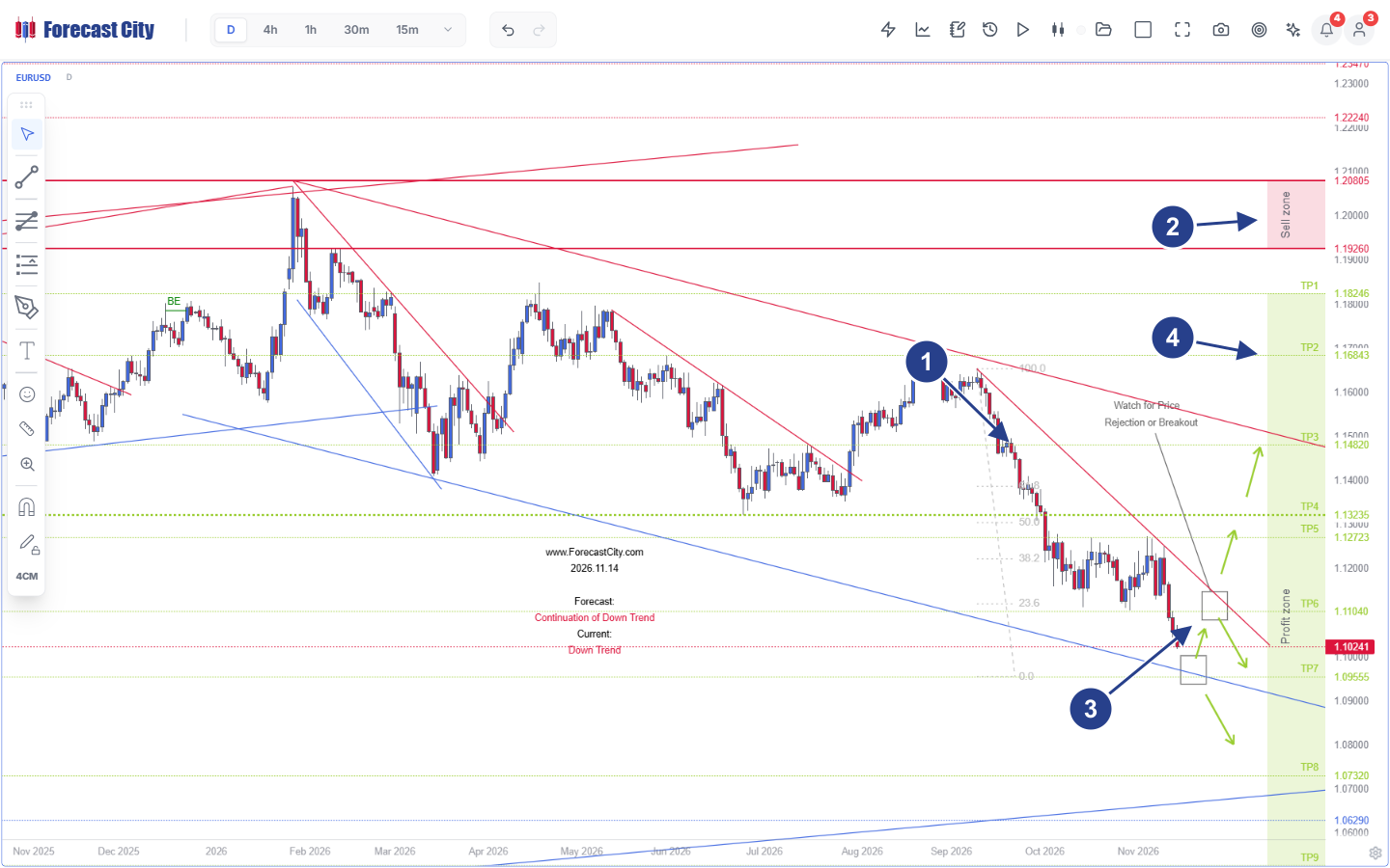
- 1Channel & Fibonacci Geometry: Multi-month descending red resistance channel from the
1.20805swing peak paired with a100.0to0.0Fibonacci retracement grid measuring corrective pullbacks. - 2Macro Sell Zone: Pink supply band spanning
1.19260to1.20805(beneath outer structural resistance at1.22240) defining the upper institutional ceiling. - 3Structural Decision Nodes: Dual
Watch for Price Rejection or Breakoutboxes at1.10241where the inner red trendline meets lower blue channel support, paired with bifurcated Green Arrows. - 4Stepped Profit Zone Ladder: Pre-computed downside objective scale running from
TP1(1.18246),TP3(1.14820), andTP6(1.11040) down throughTP7(1.09555) andTP8(1.07320).
On Figure 2, price has descended from TP1 (1.18246) through TP6 (1.11040) and compresses at 1.10241 where the inner red trendline meets the lower blue channel boundary. Whereas ten oscillators at 1.10241 pit oversold Stochastic against bearish SMA(50), Navigator AI places two explicit watch boxes (Callout 3) with bifurcated Green Arrows: bullish rejection off channel support opens a rebound toward 1.14820 (TP3), whereas a Daily close below support continues toward TP7 (1.09555) and TP8 (1.07320). Intentionally, Navigator AI draws no shaded Reverse Zone box on D, governing Daily macro anchors directly through boundary confirmations.
On execution timeframes (4h and lower), intraday shocks can breach a local threshold within one session. Figure 3 shows how Navigator AI equips Ethereum (ETHUSD 4h), trading live at 1750.79, with a two-scenario contingency plan.
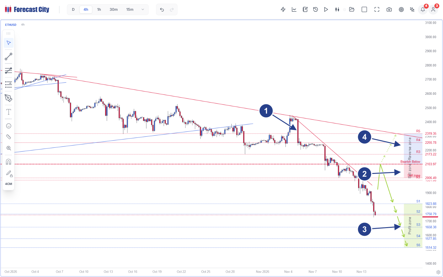
- 1Wedge Breakdown & Retest: Late-October breakdown beneath rising blue wedge support followed by the November 4 bearish rejection near
2425under dual descending red resistance trendlines. - 2Sell Zone & Falsifiable Pivot: Pink Sell zone spanning
R1(2006.49) up to the horizontal redBearish Below 2103.97Pivot invalidation line. - 3Primary Bearish Path: Solid Green Arrows projecting supply rejection from the
Sell zonedown through the green Profit zone ladder:S1(1823.88),S2(1750.79, current spot),S3(1658.38),S4(1577.85), andS5(1514.32). - 4Pre-Computed Reverse Zone: Blue-shaded Reverse zone above
2103.97plotting conditional Dashed Arrows throughR3(2173.22),R4(2255.78), andR5(2319.35) if a4hclose reclaims the Pivot.
After ETHUSD broke its rising blue wedge in late October and rejected 2425 on November 4 (Callout 1), Navigator AI anchored invalidation at Pivot = 2103.97 (Bearish Below 2103.97) above the pink Sell zone 2006.49 - 2103.97 (Callout 2). With spot sitting at S2 = 1750.79 inside the green Profit zone (Callout 3), the chart warns immediately against chasing fresh shorts 353 dollars below invalidation: disciplined execution either awaits a pullback toward 2006.49 - 2103.97 or trails existing runners toward S3 = 1658.38, S4 = 1577.85, and S5 = 1514.32. Conversely, if a confirmed 4h close reclaims 2103.97, the blue Reverse zone (Callout 4) has already mapped the alternate bullish path via Dashed Arrows through R3 = 2173.22, R4 = 2255.78, and R5 = 2319.35.
5. Conditional Stochastic Prescription and Human-in-the-Loop Supervisory Authority
Models trained solely to minimize symmetric Root Mean Square Error (RMSE) fail traders because markets impose sharply asymmetric, path-dependent loss functions. Shorting ETHUSD with a stop at 2103.97 suffers a permanent -1.0 R stop-out if a wick touches 2108.00 before dropping to 1658.38, even when average point error looks small.
Bertsimas and Kallus [1] and Lepenioti et al. [6] formalize the boundary between point estimation and prescriptive analytics. Given Synergy AI state X = 𝒰t, stochastic future trajectory Y, and flight-plan tuple z = (𝒵entry, Ppivot, {TPj}, zrev) ∈ 𝒵 under asymmetric trading loss c(z; Y), prescriptive optimization solves:
Here z*(x) is the oracle policy given X = x, ẑ(X) is Navigator AI's prescribed roadmap, z̄ is an unconditional static baseline, and 𝒫 ∈ [0, 1] is the Coefficient of Prescriptiveness.
Rather than outputting a scalar price point, z*(x) optimizes entry location relative to invalidation so pathwise stop-out distance stays tight while multi-stage targets remain open. Placing entry inside an institutional Sell zone near the Pivot converts modest directional probabilities into strongly positive R-multiple expectancy.
Verify this numerically on Figure 3 (ETHUSD 4h). A lagging EMA(20)/EMA(50) crossover confirms short late near S1 = 1823.88 against invalidation at 2103.97 (280.09 USD risk) for target S3 = 1658.38 (165.50 USD reward), yielding just 0.59 R and requiring a 62.9% win rate to break even. By contrast, Navigator AI's pullback prescription inside the Sell zone at 2040.00 risks 63.97 USD to 2103.97 while capturing 289.21 USD at S2 = 1750.79 (+4.52 R) and 381.62 USD at S3 = 1658.38 (+5.97 R), breaking even at an 18.1% win rate.
Mapped onto Sheridan and Verplank [12] and Parasuraman, Sheridan, and Wickens [10] across four automation stages (Information Acquisition, Information Analysis, Action Selection, and Action Implementation), indicator stacks strand humans at LoA 1 overload, whereas opaque black-box bots jump to brittle LoA 10 execution (see our explainability whitepaper). ForecastCity targets the aerospace co-pilot optimum: Quad-AI automates Stages 1-2 and operates Stage 3 at LoA 4 to 5, while reserving Stage 4 capital commitment for the human supervisor via AI Strategy Studio and Virtual Accounts.
6. Descriptive Indicator Stacks vs. Opaque Auto-Bots vs. Quad-AI Prescriptive Roadmaps
| Engineering Dimension | Descriptive Indicator Stack (SMA, RSI, MACD, Stoch) | Opaque Black-Box Auto-Execution Bot | 4CastMachine AI (Quad-AI) Prescriptive Roadmap |
|---|---|---|---|
| Temporal Phase Lag | Irreducible causal group delay (N - 1) / 2 bars plus nonlinear IIR phase dispersion. |
Hidden lookback sensitivity; unannounced failure on jump discontinuities. | Zero-lag exogenous NLP (Sentiment AI) fused with forward structural zone geometry. |
| Spectral Dimensionality | Severe multicollinearity: 10 oscillators collapse to erank ≈ 1.8 - 2.5 [11]. |
Overparameterized latent weights prone to in-sample snooping [4, 13]. | Orthogonal multi-modal engines (price geometry + live macro/news posteriors). |
| Multi-Timeframe Coherence | Uncoordinated across horizons; encourages 60-cell cherry-picking bias. | Typically locked to a single execution bar interval. | Hierarchical MinT coherence [14] across 9 horizons; D anchor + 4h contingencies. |
| Decision Output | Backward-looking scalar curves; zero invalidation or target geometry. | Unexplained market orders without inspectable structural stops. | Complete flight plan: Entry Zone, falsifiable Pivot, TP1-TP5+, Green & Dashed Arrows. |
| Supervisory Control [10] | LoA 1 cognitive overload and inflection-zone analysis paralysis. |
Brittle LoA 10 blind automation; high abandonment during drawdowns. |
LoA 4-5 Co-Pilot: AI prescribes roadmaps; human governs risk & capital execution. |
Frequently Asked Questions
Why does adding more oscillators to a chart worsen analysis paralysis instead of improving accuracy?
How does 4CastMachine AI overcome Bode’s causal phase-lag barrier without peeking into future bars?
Why does EURUSD Daily (D) show rejection/breakout boxes without a Reverse Zone, whereas ETHUSD 4h displays a shaded Reverse Zone?
How do prescriptive roadmaps differ from traditional buy/sell alert services or automated trading bots?
Peer-Reviewed & Industry References
- [1]Bertsimas, D., & Kallus, N. (2020). From predictive to prescriptive analytics. Management Science, 66(3), 1025-1044. https://doi.org/10.1287/mnsc.2018.3253
- [2]Corsi, F. (2009). A simple approximate long-memory model of realized volatility. Journal of Financial Econometrics, 7(2), 174-196. https://doi.org/10.1093/jjfinec/nbp001
- [3]Ehlers, J. F. (2001). Rocket Science for Traders: Digital Signal Processing Applications. New York: John Wiley & Sons.
- [4]Harvey, C. R., Liu, Y., & Zhu, H. (2016). ...and the cross-section of expected returns. The Review of Financial Studies, 29(1), 5-68. https://doi.org/10.1093/rfs/hhv059
- [5]Hyndman, R. J., Ahmed, R. A., Athanasopoulos, G., & Shang, H. L. (2011). Optimal combination forecasts for hierarchical time series. Computational Statistics & Data Analysis, 55(9), 2579-2589. https://doi.org/10.1016/j.csda.2011.03.006
- [6]Lepenioti, K., Bousdekis, A., Apostolou, D., & Mentzas, G. (2020). Prescriptive analytics: Literature review and research challenges. International Journal of Information Management, 50, 57-70. https://doi.org/10.1016/j.ijinfomgt.2019.04.003
- [7]Müller, U. A., Dacorogna, M. M., Davé, R. D., Olsen, R. B., Pictet, O. V., & von Weizsäcker, J. E. (1997). Volatilities of different time resolutions - Analyzing the dynamics of market components. Journal of Empirical Finance, 4(2-3), 213-239. https://doi.org/10.1016/S0927-5398(97)00007-8
- [8]Oppenheim, A. V., & Schafer, R. W. (2009). Discrete-Time Signal Processing (3rd ed.). Upper Saddle River, NJ: Prentice Hall.
- [9]Osler, C. L. (2003). Currency orders and exchange rate dynamics: An explanation for the predictive success of technical analysis. The Journal of Finance, 58(5), 1791-1820. https://doi.org/10.1111/1540-6261.00588
- [10]Parasuraman, R., Sheridan, T. B., & Wickens, C. D. (2000). A model for types and levels of human interaction with automation. IEEE Transactions on Systems, Man, and Cybernetics - Part A, 30(3), 286-297. https://doi.org/10.1109/3468.844354
- [11]Roy, O., & Vetterli, M. (2007). The effective rank: A measure of effective dimensionality. Proceedings of the 15th European Signal Processing Conference (EUSIPCO 2007), 606-610.
- [12]Sheridan, T. B., & Verplank, W. L. (1978). Human and Computer Control of Undersea Teleoperators. Technical Report, MIT Man-Machine Systems Laboratory, Cambridge, MA.
- [13]Sullivan, R., Timmermann, A., & White, H. (1999). Data-snooping, technical trading rule performance, and the bootstrap. The Journal of Finance, 54(5), 1647-1691. https://doi.org/10.1111/0022-1082.00163
- [14]Wickramasuriya, S. L., Athanasopoulos, G., & Hyndman, R. J. (2019). Optimal forecast reconciliation for hierarchical and grouped time series through trace minimization. Journal of the American Statistical Association, 114(526), 804-819. https://doi.org/10.1080/01621459.2018.1448825