Financial log-returns evolve as hybrid jump-diffusion semimartingales. During quiet trading hours, prices follow continuous Brownian order-book elasticity around established liquidity levels. During macroeconomic releases and geopolitical flashes, discontinuous Lévy jumps and multi-hour institutional order-flow waves dominate return variation. Any static convex combination of price-derived technical estimators and text-derived sentiment estimators is provably suboptimal across these shifting regimes. A high constant sentiment weight injects media chatter during calm diffusive sessions, whereas a high constant technical weight suffers severe deterministic filter lag during macro repricing. This paper formulates the dynamic regime-arbitration problem inside 4CastMachine AI and shows how Synergy AI continuously reweights Forecast AI (multi-timeframe price geometry and DTO candlestick probabilities) and Sentiment AI (contextual financial language modeling, standardized macro surprises, and Hawkes arrival velocity) across nine horizons from 1m to M. We derive smooth softmax gating properties, proactive pre-announcement zone expansion, and live multi-asset walkthroughs across XAUUSD, EURUSD, and BTCUSD.
1. The Structural Flaw of Static Weights Under Regime Non-Stationarity
Quantitative market architectures routinely blend technical price indicators with macroeconomic or news-sentiment scores using fixed linear weights. Whether those weights come from ordinary least squares, equal-weight averaging, or static Bayesian Model Averaging, the underlying assumption is identical. The model treats the conditional covariance between chart geometry, public text streams, and forward returns as constant across time. High-frequency market microstructure refutes that stationarity assumption in every liquid asset class.
Markets alternate between fundamentally different physical mechanisms of price discovery. Hamilton [1] demonstrated that macroeconomic time series undergo discrete structural shifts governed by latent state transitions rather than time-invariant linear autoregressions. Extending that result to dynamic asset allocation, Ang and Bekaert [2] quantified hundreds of basis points of annualized utility loss when portfolios ignore transitions between calm diffusive regimes and high-volatility shock regimes.
At intraday resolution, the contrast between quiet liquidity provision and news-driven repricing becomes even sharper. Andersen, Bollerslev, Diebold, and Vega [5] examined six years of five-minute spot foreign-exchange returns around scheduled US and European macroeconomic announcements. They defined the standardized surprise of announcement k at release timestamp t by scaling the gap between the actual print Ak,t and the pre-release institutional consensus Et-[Ak] by historical surprise dispersion σk. Unanticipated surprises trigger instantaneous jumps in the conditional mean within minutes, while conditional return volatility remains elevated for several hours. Evans and Lyons [6, 7] traced how that adjustment reaches equilibrium on institutional dealing desks. Roughly one-third of the exchange-rate shift arrives as an immediate public-information jump on the first tick, while the remaining two-thirds unfolds across subsequent trading intervals through induced institutional order flow.
Quiet trading sessions behave in the exact opposite way. When no fresh macroeconomic or corporate catalyst enters the market, unstructured financial news commentary and social streams carry very low directional precision. Tetlock [11] proved that media pessimism unbacked by new fundamental cash-flow data creates temporary price pressure that quickly mean-reverts back toward prior structural levels. Compounding that noise problem, Loughran and McDonald [12] analyzed 50,115 corporate 10-K filings and found that 73.8% of words classified as negative by standard generic dictionaries (such as liability, tax, cost, or vice) carry neutral or structural meaning in financial disclosures.
This structural dichotomy creates an inescapable mathematical dilemma for any model that combines technical and textual estimators with a constant scalar weight. Before writing the formal error bound, consider what happens physically on a chart. During a calm London morning, limit-order books are thick and price respects multi-timeframe support, resistance, and channel boundaries, while financial blogs recycle stale opinions. Minutes after a 2.8-sigma inflation surprise, trailing moving averages and oscillators still average forty-nine pre-release candles with one post-release candle, blinding pure technical filters to the new macro reality.
Let st(F)(τ) denote the horizon-τ directional estimator produced from the price filtration ℱXt, and let st(S)(τ) denote the horizon-τ estimator produced from the text and macro filtration ℱDt. Any static ensemble applies a time-invariant weight w0 ∈ [0, 1] across all market regimes Rt:
Here BF,R_t and BS,R_t denote conditional estimator biases in regime Rt, σF,R_t2 and σS,R_t2 denote conditional estimator error variances, and CovR_t denotes conditional error covariance. Under calm diffusion (BF ≈ 0, σS2 ≫ σF2), variance minimization requires w*diff ≈ σF2 / (σF2 + σS2) → 0. Immediately after a macro jump Jt_0, any causal L-bar price filter suffers deterministic lag bias |BF,jump| ∝ (1 - h0)|Jt_0|, forcing optimal weight w*jump → 1. No constant w0 can minimize conditional error in both states simultaneously.
Equation (1) says that a fixed 50/50 blend between chart analysis and news sentiment is always wrong in one half of its input. In quiet sessions (roughly 85% of trading hours), giving 50% authority to news headlines contaminates clean support and resistance levels with recycled media noise. During the 15% of hours shaped by macro shocks, giving 50% authority to backward-looking candle averages anchors the model to stale pre-announcement prices that no longer clear the order book.
A numerical check reveals the size of this error penalty. During a calm EURUSD session with orthogonal zero-bias errors, suppose the 1h technical estimator has standard error σF = 8 pips (σF2 = 64) while media sentiment carries σS = 26 pips (σS2 = 676). Equation (1) sets the optimal calm weight at w*diff = 64 / (64 + 676) = 0.086, achieving minimum MSE of 58.5 pips2 (root error 7.65 pips). A static 50/50 blend (w0 = 0.50) yields 185.0 pips2 (root error 13.60 pips), inflating error variance by 216% across quiet hours.
Now check the same pair three minutes after a 2.85-sigma US CPI shock moves equilibrium value by 60 pips. A 50-bar moving average retains 96% pre-jump prices, creating lag bias BF,jump = 57.6 pips with σF = 12 pips (BF2 + σF2 = 3,461.8 pips2). Contextual surprise parsing tracks the post-jump regime with BS,jump = 4 pips and σS = 14 pips (212.0 pips2). Optimal shock weight jumps to w*jump = 0.942, cutting MSE to 199.8 pips2, whereas keeping w0 = 0.086 explodes MSE to 2,890.5 pips2.
Hard binary calendar rules ("disable technicals for 30 minutes after CPI") fail just as badly. Unscheduled central-bank remarks, sovereign headlines, and weekend crypto liquidations never appear on an economic calendar. Worse, step-function timers create cliff-edge jumps in chart levels the instant a fixed cutoff expires.
2. Semimartingale Jump-Diffusion and Non-Parametric Regime Separation
To shift authority smoothly between technical structure and live news sentiment without arbitrary calendar timers, the engine must measure what kind of physical process is driving prices in real time. Financial asset prices do not follow pure geometric Brownian motion. Instead, continuous trading liquidity and sudden information shocks coexist on the same price tape.
We formalize log-price Xt = ln Pt on a filtered probability space (Ω, ℱ, (ℱt)t≥0, ℙ) using a regime-dependent jump-diffusion semimartingale (extending Merton [9] and Kou [9]):
Each term in Equation (2) governs a distinct layer of market behavior. The drift function μ(·) dt represents instantaneous directional pressure conditioned on recent price path Xt-Δ:t, latent market regime Rt, and active news state ℐnewst. The diffusive term σ(Rt) dWt scales a standard Brownian motion Wt by regime volatility σ(Rt), capturing normal continuous order-book matching. Finally, Jt dNt represents discontinuous price jumps of random signed amplitude Jt arriving via point process Nt.
Think of Equation (2) as decomposing every candle on your chart into two physical forces. When dNt = 0, price moves tick by tick through resting limit orders, so historical support zones, channels, and Fibonacci retracements act like elastic walls. When dNt = 1, liquidity providers pull their quotes and price teleports across empty order-book levels to reflect new macro reality.
In real markets, news shocks rarely arrive as isolated, memoryless Poisson events. A surprise Federal Reserve headline triggers immediate wire flashes, dealer desk re-hedging, Treasury yield spikes, and cross-asset margin calls, which in turn generate secondary headlines over the next hour. Hawkes [10] and Bacry, Mastromatteo, and Muzy [10] showed that this clustering behavior is accurately modeled by a self-exciting point process whose conditional arrival rate λt depends on the timing and surprise magnitude of prior events:
In Equation (3), λ0 > 0 is the quiet baseline rate of routine headlines. Each past timestamp ti carries standardized surprise |ze,i|. Parameter αH ≥ 0 sets base self-excitation, γH ≥ 0 scales amplification for major surprises, and βH > 0 sets exponential decay with half-life τ1/2 = (ln 2) / βH.
The Hawkes intensity λt works like a real-time seismograph for market shockwaves. A major surprise spikes λt instantly, and follow-on desk flashes keep it elevated while institutions digest the news. Once aftershocks stop, λt decays with half-life τ1/2 toward λ0 as order-book depth returns.
Trace Equation (3) numerically on EURUSD. Set baseline wire rate λ0 = 0.40 events per minute, αH = 0.85, γH = 0.90, and βH = 0.035 min-1, giving half-life τ1/2 = 19.8 minutes. A Core CPI surprise of |ze,1| = 2.85 at t1 = 0 lifts λt from 0.40 to 0.40 + 0.85(1 + 0.90 × 2.85) = 3.43 events per minute (an 8.58x jump). Eight secondary flashes over ten minutes push λ10 near 8.10 before smooth decay lowers it to 2.32 at t = 45 min and 0.57 by t = 120 min.
Wire velocity alone is insufficient because rumors can flood social feeds without moving institutional capital. We also test whether the price tape itself exhibits discontinuous jumps. Barndorff-Nielsen and Shephard [8] separated continuous and jump variation across MΔ intraday log-returns rt,j using Realized Variance (RVt) and Realized Bipower Variation (BVt):
In Equation (4), RVt sums squared returns and converges in probability to total quadratic variation, meaning continuous diffusive variance ∫ σu2 du plus squared jumps ∑ Ju2. By contrast, BVt multiplies adjacent absolute returns |rt,j| |rt,j-1| scaled by π / 2 ≈ 1.5708, which converges to the continuous diffusive component alone. Taking their normalized difference (with small numerical stabilizer ε = 10-10) yields the dimensionless jump-variation ratio 𝒥t ∈ [0, 1).
Why does multiplying two neighboring bars filter out jumps? If a macro shock causes a massive 50-pip jump in bar j while neighboring bars j-1 and j+1 move a normal 3 pips, squaring bar j inside RVt produces 502 = 2,500, whereas multiplying |rj||rj-1| inside BVt produces only 50 × 3 = 150. Consequently, RVt spikes far above BVt and pushes 𝒥t close to 1.0 whenever genuine jump repricing hits the tape.
Checking the numbers on twelve five-minute EURUSD bars (MΔ = 12, one trading hour) makes this concrete. If eleven bars move ±3 pips and one quiet bar moves 4 pips, then RVt = 11(9) + 16 = 115 pips2 and BVt ≈ 1.5708 × [9(9) + 2(12)] / (11/12) ≈ 114 pips2 (finite-sample adjusted), giving 𝒥t ≈ 0.01 (pure diffusion). If instead bar 7 prints a 45-pip CPI jump while all other eleven bars move ±3 pips, then RVt = 11(9) + 2,025 = 2,124 pips2, whereas BVt = 1.5708 × [9(9) + 2(45 × 3)] = 551.4 pips2. Immediately, 𝒥t = (2124 - 551.4) / 2124 = 0.740, confirming that 74% of hourly quadratic variation came from discontinuous shock repricing.
3. Continuous Softmax Regime Gating Inside Synergy AI
Inside the Quad-AI architecture of 4CastMachine AI, price structure and live news sentiment are not jammed into one monolithic black-box network. Instead, four dedicated engines separate feature extraction, modality arbitration, and prescriptive level projection into auditable stages.
First, Forecast AI computes technical state vector st(F)(τ) across all nine timeframes (1m, 5m, 15m, 30m, 1h, 4h, D, W, and M). Its inputs combine Daily Trading Opportunity (DTO) candlestick probabilities, multi-pivot support and resistance clusters, trend channels, harmonic ratios, and oscillator divergence. Second, Sentiment AI computes live macro-news state st(S)(τ) by ingesting institutional wire feeds, economic calendar surprises ze, central-bank transcripts, and cross-asset yield/currency flows through domain-adapted financial language models (resolving context-dependent polarity inversions documented by Araci [13] and Wang et al. [15]).
Synergy AI operates as the continuous arbitration layer between those two expert streams before handing unified parameters to Navigator AI. Figure 1 contrasts Synergy AI's smooth state-conditioned softmax gating network against fragile binary threshold rules.
To formalize how Synergy AI computes its continuous regime weights across horizons, we combine Dynamic Model Averaging with state-space forgetting factors (Raftery, Kárný, and Ettler [3]; Koop and Korobilis [4]) and input-conditioned Mixture-of-Experts softmax gating (Jacobs et al. [14]; Shazeer et al. [14]; Koval, Andrews, and Yan [15]). Let zt = [𝒥t, |ze,t|, λt / λ0, Δρcross,t, ψpre,t]⊤ denote the standardized regime-conditioning vector at time t. For each horizon τ ∈ {1m, ..., M}, Synergy AI evaluates:
Every symbol in Equation (5) plays a transparent architectural role. The weight wt(S)(τ) ∈ (0, 1) assigns epistemic authority to Sentiment AI on timeframe τ, while wt(F)(τ) = 1 - wt(S)(τ) assigns the complementary authority to Forecast AI. The term ℓDMAm,t|t-1(τ) is the exponentially forgotten cumulative out-of-sample log-likelihood score of expert m over recent bars with horizon-specific forgetting factor ατ ∈ [0.94, 0.995]. The inner product θm,τ⊤ zt projects the live jump-and-news regime vector zt onto expert m, and Tτ > 0 is the horizon temperature parameter controlling transition smoothness.
Equation (5) acts like an experienced institutional head of desk managing two specialists: a master chartist (Forecast AI) and a central-bank macro wire analyst (Sentiment AI). On quiet days when zt is near zero, the softmax gate listens 82% to the chartist. The second a genuine surprise spikes both 𝒥t and λt, the gate smoothly hands 75%-88% of intraday authority to the macro specialist, then gradually returns control to the chartist as order-book liquidity refills.
Although exact production parameter matrices remain proprietary to 4CastMachine AI, Equation (5) guarantees two rigorous mathematical properties on live charts:
- Lipschitz Smoothness Without Flicker: Defining the log-odds differential Δuτ(zt) = [(ℓS - ℓF) + (θS,τ - θF,τ)⊤ zt] / Tτ, Equation (5) reduces to wt(S)(τ) = (1 + exp(-Δuτ))-1, whose derivative with respect to Δuτ is strictly bounded above by 1/4. Small tick fluctuations in realized variance never cause forecasted zones to snap erratically between states.
- Spectral Horizon Separation: Gating sensitivity norms scale inversely with candle duration: ‖θS,5m - θF,5m‖ > ‖θS,15m - θF,15m‖ > ‖θS,1h - θF,1h‖ > ‖θS,4h - θF,4h‖ > ‖θS,D - θF,D‖ > ‖θS,W - θF,W‖. A single monthly CPI release sharply shifts
5m,15m, and1hintraday roadmaps without overturningWorMmacro trend structure unless cumulative data alters the multi-quarter interest-rate cycle.
A numerical check illustrates both properties simultaneously. Suppose that on a quiet morning with T1h = 1.0 and TW = 1.25, baseline DMA log-odds favor technical structure at ℓS - ℓF = -1.65 on 1h and -2.20 on W, while calm microstructure adds +0.13 on 1h and +0.05 on W. Evaluating Equation (5) gives wt(S)(1h) = (1 + exp(1.52))-1 = 0.179 (82.1% Forecast AI) and wt(S)(W) = (1 + exp(2.15 / 1.25))-1 = 0.152 (84.8% Forecast AI). At t0 of a 2.85-sigma CPI surprise (𝒥t = 0.78, λt / λ0 = 8.6), the 1h projection surges by +2.98 (bringing net logit to +1.33), smoothly lifting wt_0(S)(1h) = (1 + exp(-1.33))-1 = 0.791. Meanwhile, the Weekly projection adds only +0.76, nudging wt_0(S)(W) modestly to 0.240 so long-horizon structural geometry stays anchored.
Figure 2 plots this full 240-minute impulse-response trajectory alongside the resulting cumulative out-of-sample conditional log-density score.
0.18 to 0.79 at announcement timestamp t0 and relaxing exponentially with half-life τ1/2 as institutional liquidity replenishes, while Forecast AI weight wt(F) = 1 - wt(S) regains structural authority. Panel B compares cumulative out-of-sample conditional log-score gains across Synergy AI, a static 50/50 blend, and pure backward-looking technical filters.Synergy AI also addresses a critical microstructure hazard before scheduled tier-one news prints. Seconds prior to a major release such as US CPI, FOMC, or Non-Farm Payrolls at scheduled timestamp Tk, electronic market makers withdraw resting limit orders near spot price. That liquidity vacuum routinely produces a violent two-way initial whip (often 2x to 3x quiet-session range) before institutional directional flow settles. Leaving quiet-session support or resistance zones unadjusted right next to spot exposes intraday setups to mechanical sweep losses.
To prevent premature sweeps, Sentiment AI and Synergy AI maintain the empirical distribution ℰ(k)(ℳ) of historical initial announcement excursions for event class k on symbol ℳ. Inside the pre-announcement window t ∈ [Tk - Δpre, Tk], Navigator AI displaces and widens its forecasted Buy Zone and Sell Zone buffers outward according to:
In Equation (6), dtech,t(τ) is the normal diffusive distance from spot price to the technical zone boundary on timeframe τ, and Qα(ℰ(k)(ℳ)) is the historical α-quantile excursion (for example, the 85th-percentile initial release sweep) recorded for that specific macro report on symbol ℳ. The smooth ramp ψpre(u) ∈ [0, 1] rises toward 1.0 as t → Tk, and κτ scales sensitivity by timeframe.
Equation (6) encodes practical institutional risk hygiene directly into chart geometry. If quiet-session Gold support sits $12 below spot, yet FOMC statements historically whip Gold $29.50 in the first thirty seconds, keeping a $12 Buy Zone invites a liquidity-vacuum stop-out. Moving trading zones farther based on that release's historical shock range places the zone outside the initial bid-ask vacuum.
Numerically, suppose spot Gold (XAUUSD) trades at 2642.00 twenty minutes before an FOMC rate decision (ψpre = 1.0, κ1h = 1.0), with quiet technical zone distance dtech,t(1h) = $14.00 (2628.00) and historical 85th-percentile FOMC initial sweep Q0.85 = $29.50. Equation (6) expands the zone displacement to dzone,t(1h) = 14.00 + 1.0 × max(0, 29.50 - 14.00) = $29.50, shifting the outer boundary down to 2612.50 ahead of the 18:00 UTC print.
4. Static Technicals vs. Pure NLP Sentiment vs. Synergy AI
Evaluating single-modality technical systems, standalone NLP news feeds, and Synergy AI side by side clarifies why neither chart geometry nor text sentiment can stand alone across a full trading week. Each row in the matrix below isolates a distinct market regime and traces the operational consequence on live price levels.
| Regime / Criterion | Static Technical Filters (EMA, RSI, MACD) | Standalone NLP Sentiment Stream | Synergy AI Continuous Regime Gating |
|---|---|---|---|
| Calm Diffusive Trend (𝒥t ≈ 0) | Tracks trend with (L-1)/2 bar filter lag; respects support elasticity. | High false-reversal rate from unbacked media chatter (Tetlock [11]). | Forecast AI dominant: suppresses low-credibility chatter; preserves crisp structural Buy/Sell Zones. |
| Equilibrium Range | Moving-average crossovers whipsaw repeatedly inside horizontal bounds. | Polarity swings erratically on recycled headlines without price anchors. | Balanced structural bounds: anchors range boundaries while monitoring catalyst buildup in zt. |
| Pre-Release Window (Tk - 30m) | Blind to upcoming CPI or FOMC shock; leaves tight levels inside sweep range. | Flags calendar timestamp but projects no price-space buffer geometry. | Proactive zone expansion: moves Buy/Sell Zones farther by historical report excursion Qα(ℰ(k)). |
| Tier-1 Macro Jump (|ze| > 2σ) | Severe lag bias; oscillators misread order-flow breakout as "oversold/overbought". | Captures surprise polarity instantly but lacks chart invalidation coordinates. | Sentiment AI surge on 5m-1h: updates intraday outlook; activates Reverse Zone dashed path if Pivot breaks. |
| Post-Shock Decay (λt → λ0) | Requires 15-50 bars to flush stale pre-shock prices from trailing windows. | Lingers on repetitive post-event commentary after institutional flow finishes. | Smooth DMA relaxation: decays wt(S)(τ) with half-life τ1/2 back toward Forecast AI structure. |
5. Live Multi-Timeframe Evidence & Multi-Asset Walkthroughs
To observe spectral horizon separation on an actual production workspace, Figure 3 captures spot Gold (XAUUSD) on 4CM-AI Charts alongside the live 4CastMachine AI multi-timeframe panel spanning 15m through M.
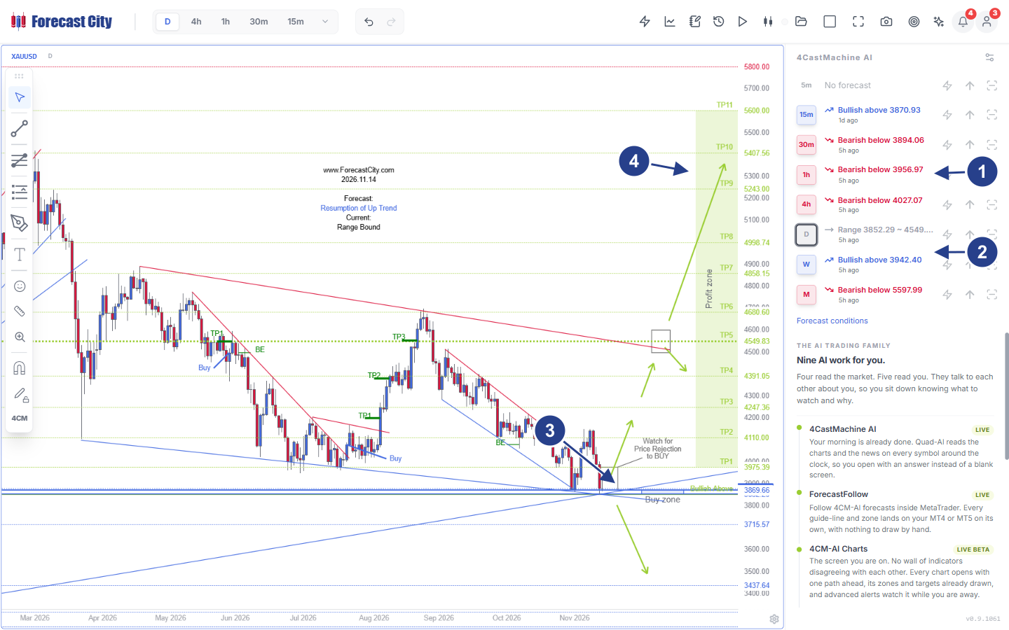
- 1Short-Horizon Bearish Stack: Intraday horizons reflect downward corrective flow (
30m Bearish below 3894.06,1h Bearish below 3956.97,4h Bearish below 4027.07), while micro15mstabilizes atBullish above 3870.93. - 2Macro Structural Horizons: Daily reads
Range 3852.29 ~ 4549.83(Forecast: Resumption of Up Trend | Current: Range Bound), Weekly holdsBullish above 3942.40, and Monthly caps macro resistance atBearish below 5597.99. - 3Daily Buy Zone & Structural Floor: Price tests the converging multi-month wedge apex right at the
Buy zoneandBullish Above 3869.66boundary (Watch for Price Rejection to BUY), backed by deeper supports at3715.57and3437.64. - 4Multi-Stage Profit Zone Ladder: Primary upside trajectory projects stepped structural targets from
TP1 3975.39throughTP5 4549.83(upper wedge boundary) up to macro extensionTP11 5600.00.
Trace the numerical hierarchy visible in Figure 3. Gold pulled back from its September peak inside a descending red channel toward multi-month ascending blue support. On intermediate horizons (marker 1), corrective order flow keeps 30m (Bearish below 3894.06), 1h (Bearish below 3956.97), and 4h (Bearish below 4027.07) aligned downward until price reclaims those pivots. Yet right at the Daily Buy zone near 3869.66, 15m already turned Bullish above 3870.93 as buyers absorbed supply.
Now inspect the macro rows (marker 2) and Daily canvas (markers 3 and 4). Because Synergy AI enforces monotonic horizon scaling (‖Θ1h‖ > ‖Θ4h‖ > ‖ΘD‖ > ‖ΘW‖), intraday drift on 1h and 4h never overwrites Daily or Weekly structure. Daily reads Current: Range Bound inside 3852.29 ~ 4549.83 with Forecast: Resumption of Up Trend above Bullish Above 3869.66, while Weekly holds Bullish above 3942.40 beneath macro ceiling M Bearish below 5597.99. The chart instructs Watch for Price Rejection to BUY at the Buy zone. Confirmed rejection projects the stepped Profit zone ladder through TP1 3975.39, TP2 4110.00, TP3 4247.36, TP4 4391.05, and upper-wedge decision node TP5 4549.83 up to TP11 5600.00. Conversely, a decisive Daily close below the floor exposes lower structural supports at 3715.57 and 3437.64.
Two cross-asset scenarios illustrate the same continuous gating equations on spot FX and 24/7 crypto venues.
During a quiet Wednesday London-New York overlap at 13:30 UTC, EURUSD trades at 1.08820 above its 1h Pivot (Bullish Above 1.08500), with Buy Zone 1.08500-1.08640 and ATR(264, D) = 68 pips. Realized variance (0.92 × 10⁻⁶) matches bipower variation (0.86 × 10⁻⁶), giving 𝒥t = 0.065. Synergy AI holds wt(S)(1h) = 0.18, keeping 82% weight on Forecast AI so social-media dollar chatter never distorts the pullback zone.
Ahead of Thursday 12:30 UTC US Core CPI, the 85th-percentile 15m CPI excursion (Q0.85 = 54 pips) triggers Equation (6) zone widening. When Core CPI prints +0.4% MoM vs. +0.2% consensus (ze = +2.85), EURUSD drops 62 pips in five minutes to 1.08200. Trailing EMA(50) sits stuck at 1.08740 while RSI(14) = 21.4 lures static bots into buying against institutional USD flow [7]. Inside Quad-AI, 𝒥t = 0.78 lifts wt(S)(15m) → 0.86 and wt(S)(1h) → 0.79 (Daily shifts modestly to 0.38). Closing below 1.08500 across the Reverse Zone activates dashed downside arrows toward S3 = 1.07950 and S4 = 1.07720.
BTCUSD trades 24/7 on venues where Saturday order-book depth thins by 40% to 60%. With spot at 80450.00 above its 1h Pivot (78894.89, Buy Zone 78894.89-79703.62) and 8h funding crowded at +0.042%, an unscheduled Saturday 21:14 UTC regulatory headline triggers 14 follow-on wire flashes in nine minutes (λt / λ0 = 7.2) and $380M in long liquidations (𝒥t = 0.83). Calendar rules are blind on Saturday night, whereas Synergy AI drives wt(S)(15m) → 0.89 immediately. Following ForecastCity Academy execution rules, waiting for closed-candle confirmation avoids blind limit fills at 79700; once a 15m candle closes below 78894.89, Reverse Zone dashed arrows map continuation toward 75733.49.
Practitioners can inspect live multi-horizon roadmaps across more than 200 symbols on 4CM-AI Charts, review visual step-by-step multi-engine lessons in the ForecastCity Academy, and examine the complete empirical literature list on the Academy Sources & Bibliography page.
Frequently Asked Questions
Does Synergy AI use a binary calendar switch during CPI, FOMC, or NFP releases?
Why do 5m and 1h roadmaps react faster to breaking news than W and M roadmaps?
How does 4CastMachine AI protect intraday setups right before scheduled economic news?
Why do lagging oscillators like RSI and EMA fail during macro surprise jumps?
How should a trader read cross-timeframe disagreement in the 4CastMachine AI panel?
Peer-Reviewed & Industry References
- [1]Hamilton, J. D. (1989). A New Approach to the Economic Analysis of Nonstationary Time Series and the Business Cycle. Econometrica, 57(2), 357-384. https://doi.org/10.2307/1912559
- [2]Ang, A., & Bekaert, G. (2002). International Asset Allocation With Regime Shifts. The Review of Financial Studies, 15(4), 1137-1187. https://doi.org/10.1093/rfs/15.4.1137
- [3]Raftery, A. E., Kárný, M., & Ettler, P. (2010). Online Prediction Under Model Uncertainty via Dynamic Model Averaging: Application to a Cold Rolling Mill. Technometrics, 52(1), 52-66. https://doi.org/10.1198/TECH.2009.08104
- [4]Koop, G., & Korobilis, D. (2012). Forecasting Inflation Using Dynamic Model Averaging. International Economic Review, 53(3), 867-886. https://doi.org/10.1111/j.1468-2354.2012.00704.x
- [5]Andersen, T. G., Bollerslev, T., Diebold, F. X., & Vega, C. (2003). Micro Effects of Macro Announcements: Real-Time Price Discovery in Foreign Exchange. American Economic Review, 93(1), 38-62. https://doi.org/10.1257/000282803321455151
- [6]Evans, M. D. D., & Lyons, R. K. (2002). Order Flow and Exchange Rate Dynamics. Journal of Political Economy, 110(1), 170-180. https://doi.org/10.1086/324391
- [7]Evans, M. D. D., & Lyons, R. K. (2008). How Is Macro News Transmitted to Exchange Rates? Journal of Financial Economics, 88(1), 26-50. https://doi.org/10.1016/j.jfineco.2007.06.001
- [8]Barndorff-Nielsen, O. E., & Shephard, N. (2004). Power and Bipower Variation with Stochastic Volatility and Jumps. Journal of Financial Econometrics, 2(1), 1-37. https://doi.org/10.1093/jjfinec/nbh001
- [9]Merton, R. C. (1976). Option Pricing When Underlying Stock Returns Are Discontinuous. Journal of Financial Economics, 3(1-2), 125-144 (DOI); & Kou, S. G. (2002). A Jump-Diffusion Model for Option Pricing. Management Science, 48(8), 1086-1101 (DOI).
- [10]Hawkes, A. G. (1971). Spectra of Some Self-Exciting and Mutually Exciting Point Processes. Biometrika, 58(1), 83-90 (DOI); & Bacry, E., Mastromatteo, I., & Muzy, J.-F. (2015). Hawkes Processes in Finance. Market Microstructure and Liquidity, 1(1), 1550005 (DOI).
- [11]Tetlock, P. C. (2007). Giving Content to Investor Sentiment: The Role of Media in the Stock Market. The Journal of Finance, 62(3), 1139-1168. https://doi.org/10.1111/j.1540-6261.2007.01232.x
- [12]Loughran, T., & McDonald, B. (2011). When Is a Liability Not a Liability? Textual Analysis, Dictionaries, and 10-Ks. The Journal of Finance, 66(1), 35-65. https://doi.org/10.1111/j.1540-6261.2010.01625.x
- [13]Araci, D. (2019). FinBERT: Financial Sentiment Analysis with Pre-trained Language Models. arXiv preprint arXiv:1908.10063. https://doi.org/10.48550/arXiv.1908.10063
- [14]Jacobs, R. A., Jordan, M. I., Nowlan, S. J., & Hinton, G. E. (1991). Adaptive Mixtures of Local Experts. Neural Computation, 3(1), 79-87 (DOI); & Shazeer, N., et al. (2017). Outrageously Large Neural Networks: The Sparsely-Gated Mixture-of-Experts Layer. ICLR 2017, arXiv:1701.06538.
- [15]Wang, X.-L., et al. (2024). From News to Forecast: Integrating Event Analysis in LLM-Based Time Series Forecasting with Reflection. NeurIPS 2024 (arXiv:2409.17515); & Koval, R., Andrews, N., & Yan, X. (2025). Multimodal Language Models with Modality-Specific Experts for Financial Forecasting. arXiv:2509.19628.